Data abstraction
In the previous post we discussed why you should care about data visualization. In this one we will start looking more in detail at data, so that we can develop the tools to choose at an appropriate graph.
Data can come into many different flavors, and here we will take a look at how we can classify them depending on their qualities and on our previous knowledge.
Data formats
In the simplest case our dataset will consist into a collection of items, and each item will have a set of attribute.
In this case we are dealing with a tabular dataset. A more involved case is the one we also have relationships between the items, and in this case we are working with a network.
There are also more involved kinds of datasets, which we won’t discuss here for now. Some examples are field datasets, where one displays the value of a certain quantity for each point of a discretized space, or geometry dataset, where one has a collection of shapes belonging to some space. Field datasets are very common when one deals with weather maps or topography maps, while an example of geometry dataset is given by a street map or by the map of the regions or of the cities of a certain country.
For the moment we will only focus on tabular datasets. A tabular dataset can be represented, as the name suggests, with a table:
| item | attribute 1 | attribute 2 | … | attribute N |
|---|---|---|---|---|
| 1 | $a_1$ | $b_1$ | … | $z_1$ |
| 2 | $a_2$ | $b_2$ | … | $z_2$ |
| 3 | $a_3$ | $b_3$ | … | $z_3$ |
| … | … | … | … | … |
| M | $a_M$ | $b_M$ | … | $z_M$ |
Each attribute can be classified in a large number of ways, and here we will only discuss the main ones.
Here we will mostly follow Tamara Munzner’s textbook Visualization Analysis and Design.
Attribute types
Attribute types define the mathematical operations that makes sense to do on an attribute.
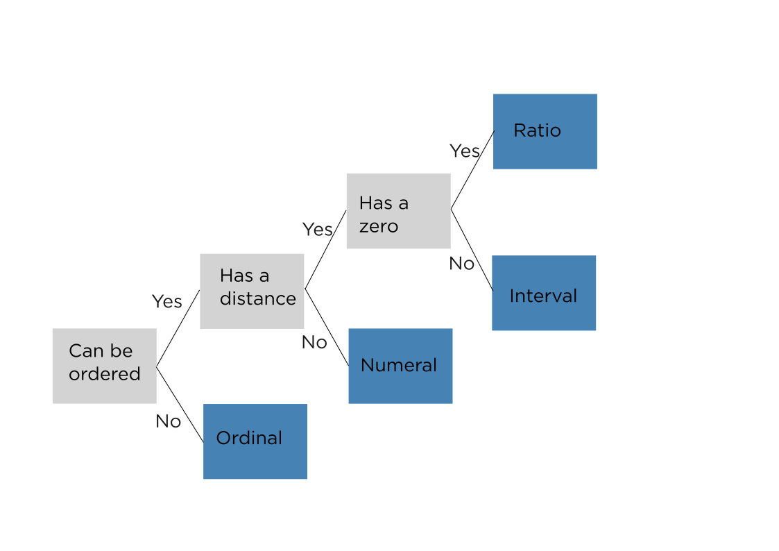
If an attribute doesn’t have a natural order we call it categorical or nominal.
Examples of nominal attributes are
- City names
- Gender (assuming it’s a discrete quantity).
- Eye color
If an attribute has a natural order but we can’t define a distance between their values we say it’s ordinal.
Ordinal attributes are
- Grade
- Education level
- Sport ranking
In this case, it doesn’t makes sense to sum, subtract or do any other arithmetic operations over the attribute.
If our attribute comes with a concept of distance we have quantitative attributes.
Quantitative attributes can be further sub-classified depending if they have a natural zero or not. Attributes which don’t have a natural zero are called interval attributes, while those which have are named ratio attributes.
Example of interval attributes are
- Temperatures expressed in Fahrenheit or Celsius degrees
- pH
While ratio attributes are:
- Temperatures expressed in Kelvin degrees
- Length
- Mass
- Any percentage
- Earnings (where negative earning means loss)

Moreover, we can also classify any ordered attribute attribute depending on the possible range of values it can take.
- A sequential attribute is an attribute which can take any value between a minimum and a maximum. Examples of sequential attributes are the day of the week as well as height or weight.
- A diverging attribute is an attribute which can be decomposed into two directions, a positive one and a negative one. Examples of diverging attributes are hours of the day (AM/PM), latitude (North/South) or elevation (above or below the sea level).
Finally, a cyclic attribute is an attribute where the minimum possible value corresponds to the maximum possible value. Examples of cyclic attributes are longitude, hour of the day and day of the week.
From our examples you may have noticed that a cyclic attribute can be either sequential, as the hour of the day, or diverging, as the longitude.
Attribute semantics
The mathematical operations we can perform with an attribute isn’t of course the only meaningful way we can classify the data. Another very important aspect of an attribute that we should consider when choosing how to visualize an attribute is its meaning. The semantic classification I found more useful in my personal experience is the one used by Tamara Munzner in her textbook .
| Semantic | Meaning | Example |
|---|---|---|
| Key vs Value | A key attribute is used to identify an element, a value attribute does not | City name vs city population, date vs temperature |
| Spatial | Our attribute has a geographical connotation | zip code, latitude, city name |
| Temporal | Our attribute is associated with time | seconds, day of the week |
| Hierarchical | Two or more attributes have a natural hierarchy | year, month, day, hour but also continent, country, city |
Conclusions
Before deciding how to visualize your dataset you must first of all consider what are the types of the attribute you want to visualize and whether they have some special connotation. Here we have seen how to determine the attribute type and the most common attribute semantic. In the next post we will discuss some of the most common visualizations associated with each data type.
Suggested readings
- Munzner, T. (2015). Visualization Analysis and Design. CRC Press. ISBN: 9781498759717
