

Point patterns
The last missing type of analysis is point pattern analysis, where we recall that in this kind of analysis the domain of the stochastic process underlying the data generation is random itself.
In order to tackle this kind of problem, we will use a Poisson point process, where we first divide our region of interest into small sub-regions, and we assume that the number of events in each sub-region is governed by a Poisson process:
\[y_j \sim Poisson(\mu_j)\,.\]Moreover, we assume that
\[\mu_j \propto \int_{\Omega_j} dx dy e^{\lambda(x, y)}\,.\]The dataset
We will use the Gorillas dataset provided in the spatstat R package. The R version of this exercise can be found in this very nice blog, where you can also find some interesting literature.
from matplotlib import pyplot as plt
import pandas as pd
import geopandas as gpd
import numpy as np
import pymc as pm
import arviz as az
import seaborn as sns

from delaunay_refine.triangulation import triangulation_from_gdf

gdf_full = gpd.read_file('/home/stippe/Downloads/gorillas/gorillas.shp')

gdf = gdf_full[gdf_full['season']=='dry']

fig, ax = plt.subplots()
gdf.plot(ax=ax)
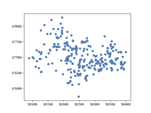
Let us now triangulate our space. We will first introduce a small buffer in order to ensure that all the points are inside our relevant region, we will then perform a constrained Delaunay triangulation, and we will finally refine it in order to obtain a thin enough triangulation. In order to do so, I will use the delaunay-refine package, which I implemented. There are other python packages which are better from a mathematical point of view, but I preferred implementing it from scratch in order to keep everything under control. Finding a good triangulation is crucial, since large triangles may introduce large errors in the computation of the integral, while having too many triangles will let your computational time explode.
tri_base = gdf.delaunay_triangles()
gdf_bds = gpd.GeoDataFrame(geometry=[tri_base.union_all().buffer(500)],
                           crs=tri_base.crs
                           ).simplify_coverage(
    tolerance=200).constrained_delaunay_triangles().explode()

tri = triangulation_from_gdf(gdf_bds)

min_angle = 18
max_area = 2e4
min_area = 0.5e4


tri.refine(min_angle=min_angle, max_area=max_area, min_area=min_area)
gdf_tri = tri.to_gdf(crs=gdf.crs)
gdf_tri['id'] = range(len(gdf_tri))

fig, ax = plt.subplots()
gdf_tri.boundary.plot(color='lightgray', lw=1, ax=ax)
gdf.plot(ax=ax, marker='x')
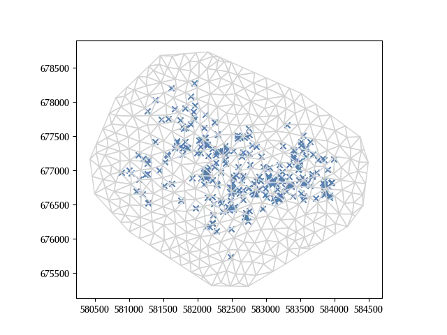
Our triangulation looks satisfactory, especially in the internal region, where we are more interested in getting a reliable estimate.
We should keep in mind that the triangulation should be dense enough to allow the approximation of a constant GP over the triangle, and the best way to check this is to verify that a thinner triangulation gives the same result.
We can now prepare the dataset for our model. In order to fit our model, we will use a gaussian process with a Matern 5/2 covariance kernel. In order to make our life simpler, we will center and scale the coordinates.
gdf_n = gdf_tri.sjoin(gdf, predicate='contains', how='left')
gdf_fit = gdf_n.dissolve(by='id', aggfunc='count')

X0 = np.array([gdf_fit.centroid.x, gdf_fit.centroid.y]).T

X0_mean = np.mean(X0, axis=0)
X0_scale = 1e3
Xv = (X0-X0_mean)/X0_scale

with pm.Model(coords={'id': range(len(gdf_fit)), 'dim': ['x', 'y']}) as model:
    X = pm.Data('X', Xv, dims=('id', 'dim'))
    lam = pm.Normal('lam', sigma=3)
    eta = pm.Normal('eta', 5)
    phi = pm.Exponential('phi', 2)
    gp = pm.gp.HSGP(m=[10, 10], L=[2.2, 2.2], cov_func=eta**2*pm.gp.cov.Matern52(2, ls=phi))
    beta = gp.prior('beta', X=X, dims=('id'))
    xi = pm.Deterministic('xi', lam + beta, dims=('id'))
    mu = pm.Deterministic('mu',  pm.math.exp(xi)*gdf_fit.area/1e5, dims=('id'))
    y = pm.Poisson('y', mu=mu, observed=gdf_fit['index_right'], dims=('id'))

rng = np.random.default_rng(42)

kwargs=dict(draws=1500, tune=1500, nuts_sampler='nutpie', rng=rng, target_accept=0.85)

with model:
    idata = pm.sample(**kwargs)

az.plot_trace(idata, var_names=['lam', 'eta', 'phi'])
fig = plt.gcf()
fig.tight_layout()
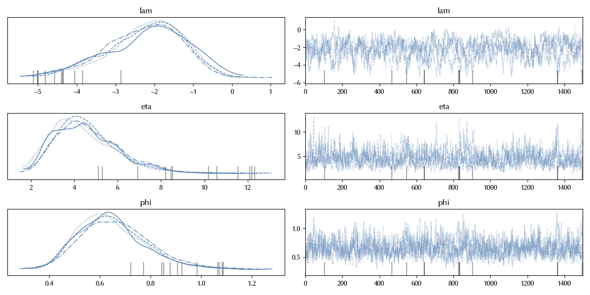
The trace is not perfect, but since this model is quite time-demanding, we won’t use a longer trace. In the above model, we choose $L=[2.2, 2.2]$ since the data roughly span the range $[-2, 2].$
Let us now compare the results of our model with the data.
gdf_est = gdf_fit.copy()

gdf_est['xi'] = idata.posterior['xi'].mean(dim=('draw', 'chain'))
gdf_est['mu'] = idata.posterior['mu'].mean(dim=('draw', 'chain'))

fig, ax = plt.subplots()
gdf_est.plot('xi', ax=ax)
gdf.plot(ax=ax, marker='x', color='gray', alpha=0.6)
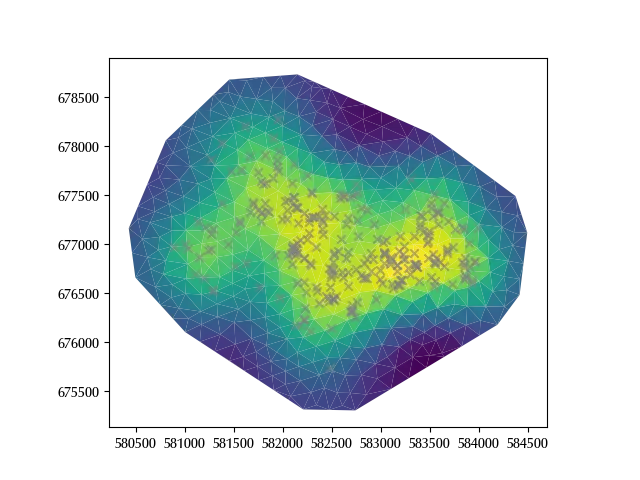
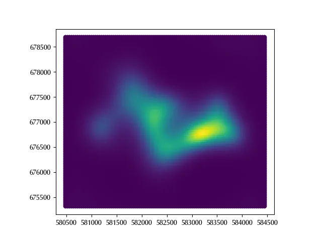
The result seems reasonable, since a higher value of the parameter corresponds to a larger density of points. We can now use our model to compute the probability at any point in the vicinity of our data.
xpl = np.linspace(Xv.T[0].min(), Xv.T[0].max(), 100)
ypl = np.linspace(Xv.T[1].min(), Xv.T[1].max(), 100)

mgrid = np.meshgrid(xpl, ypl)

Xv_pred = np.array([mgrid[0].reshape(-1), mgrid[1].reshape(-1)]).T

model.add_coords({'id_pred': range(len(Xv_pred))})

with model:
    X_pred = pm.Data('X_pred', Xv_pred, dims=('id_pred', 'dim'))
    beta_pred = gp.conditional('beta_pred', Xnew=X_pred, dims=('id_pred'))
    xi_pred = pm.Deterministic('xi_pred', lam + beta_pred, dims=('id_pred'))

with model:
    idata_pred = pm.sample_posterior_predictive(idata, var_names=['beta_pred', 'xi_pred'])

xy_pred = (X0_mean+X0_scale*Xv_pred).T

gdf_pp = gpd.GeoDataFrame(crs=gdf.crs, geometry=gpd.points_from_xy(xy_pred[0], xy_pred[1]))

gdf_pp['xi'] = np.exp(idata_pred.posterior_predictive['xi_pred']).mean(dim=('draw', 'chain'))

fig, ax = plt.subplots()
gdf_pp.plot('xi', ax=ax)
Conclusions
Poisson point processes are very common in many different fields, from biology to geophysics, and they can be easily implemented with little work thanks to PyMC.
%load_ext watermark
%watermark -n -u -v -iv -w -p xarray
Python implementation: CPython
Python version : 3.12.8
IPython version : 8.31.0
xarray: 2025.1.1
matplotlib : 3.10.6
pandas : 2.3.1
arviz : 0.21.0
seaborn : 0.13.2
delaunay_refine: 0.1.0
pymc : 5.22.0
geopandas : 1.1.1
numpy : 2.2.6
Watermark: 2.5.0