

Geostatistical data
As we previously anticipated, geostatistical data is spatial data such that the spatial domain is a continuous subset of $\mathbb{R}^d$ (in our case $d=2$). Since we generally cannot observe the data for an infinite amount of points, so we need to rely on some kind of model in order to interpolate the data, and this procedure is known as kriging, which is nothing but GP regression.
GP regression is already implemented in many libraries, but we will use PyMC for this task, since it enables us to fully customize our model.
For this problem we will use the Meuse river dataset, which is a quite well known dataset in the context of geostatistics.
The dataset can be easily found online, and as explained in this web page the coordinates are expressed into the EPSG:28992 or Amersfoort crs, which is a quite common CRS when dealing with Dutch data. The dataset is multivariate, and it can be used to perform regression with respect to non-spatial data too, but since we want to focus on kriging, we will only consider the spatial (x and y) variables.
import pandas as pd
import geopandas as gpd
import numpy as np
import rioxarray as rxr
import xarray as xr
import pymc as pm
import arviz as az
import seaborn as sns
from matplotlib import pyplot as plt

rng = np.random.default_rng(42)

df = pd.read_csv('https://raw.githubusercontent.com/filipkral/meuse/refs/heads/master/meuse.txt')

gdf = gpd.GeoDataFrame(df, crs=28992, geometry=gpd.points_from_xy(df['x'], df['y']))

fig, ax = plt.subplots()
gdf.plot('lead', ax=ax)
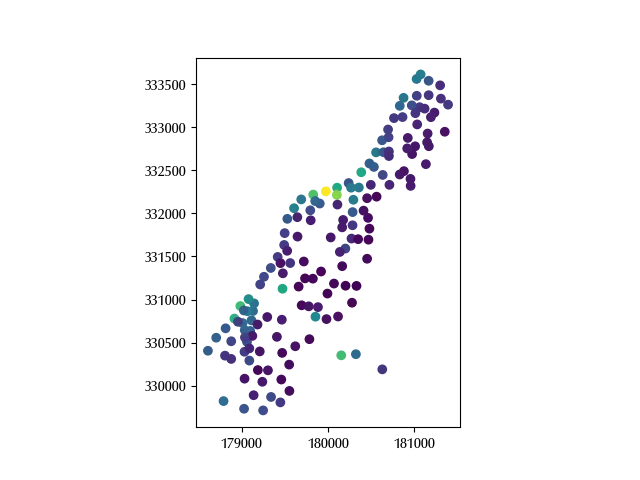
Let us first of all translate and scale the data. Before performing these operations, a comment is needed in order to clarify one of the steps. A common (and quite reasonable) assumption used in kringing is that the kernel only depends on the distance between points, and this makes quite a lot of sense, if the two spatial coordinates are expressed in the same physical unit. In order to keep this invariance, when we scale the coordinates, we must scale both of them in the same way.
Before setting up the prior, let us take a look at the data
np.log(gdf['lead']).max()
We can assume a normal distribution with zero mean and variance equal to 10 for the prior of the average, while we will assume an exponential distribution with mean equal to 10 for the data variance.
For the GP part, we will assume a zero mean GP process with Matern 5/2 kernel and this will ensure us the continuity up to the second derivative. For the GP multiplicative scale, we will take an exponential with mean equal to 2, while for the GP length we will take a Gamma distribution with mean and variance equal to 1/2 and 1 respectively.
X_full = gdf[['x', 'y']]

mn = X_full.mean(axis=0)
sg = np.max(X_full.std(axis=0))*2

X = (X_full - mn)/sg

with pm.Model(coords={'feature': ['x', 'y'], 'cols': ['elev', 'dist'], 'obs': np.arange(len(gdf))}) as model:
    Xv = pm.Data('X', X, dims=('obs', 'feature'))
    alpha = pm.Normal('alpha', mu=0, sigma=10)
    # beta = pm.Normal('beta', mu=0, sigma=2, dims=('cols'))
    rho = pm.Exponential('rho', 0.5)
    eta = pm.Gamma('eta', mu=0.5, sigma=1)
    gp = pm.gp.HSGP(m=[25, 25], L=[1.2, 1.2], cov_func=rho*pm.gp.cov.Matern52(2, ls=eta))
    phi = gp.prior('phi', X=Xv, dims=('obs'))
    mu = pm.Deterministic('mu', alpha+phi, dims=('obs'))
    sigma = pm.Exponential('sigma', 0.1)
    y = pm.Normal('y', mu=mu, sigma=sigma, observed=np.log(gdf['lead']), dims=('obs'))

with model:
    prior_pred = pm.sample_prior_predictive(random_seed=rng)

fig, ax = plt.subplots()
az.plot_ppc(prior_pred, group='prior', ax=ax)

Our guess seems quite appropriate for the data. Let us now fit the model.
with model:
    idata = pm.sample(nuts_sampler='numpyro', random_seed=rng)

az.plot_trace(idata, var_names=['alpha', 'sigma', 'rho', 'eta'])
fig = plt.gcf()
fig.tight_layout()
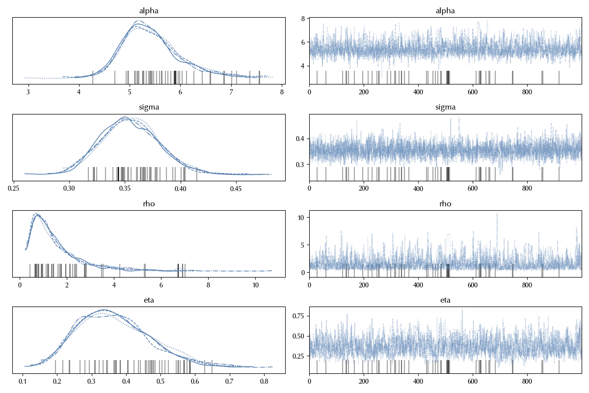
The trace of the above variable look fine, and the GP process variables look ok too
az.summary(idata, var_names=['phi'])['r_hat'].max()
Let us now compare our prediction for the average with the data, and to do so we will predict the log-mean parameter on a raster dataset.
xv = np.arange(X.min().values[0]-1e-3, X.max().values[0]+1e-2, 0.03)
yv = np.arange(X.min().values[1]-1e-3, X.max().values[1]+1e-3, 0.03)

Xmesh = np.meshgrid(xv, yv)

Xpred = np.vstack([Xmesh[0].ravel(), Xmesh[1].ravel()]).T

model.add_coord('obs_pred', values=np.arange(len(Xpred)))

with model:
    Xvpred = pm.Data('Xpred', Xpred, dims=('obs_pred', 'feature'))
    phi_pred = gp.conditional('phi_pred', Xnew=Xvpred, dims=('obs_pred'))
    mu_pred = pm.Deterministic('mu_pred', alpha+phi_pred, dims=('obs_pred'))

with model:
    idata_new = pm.sample_posterior_predictive(idata,
                                               var_names=['phi_pred', 'mu_pred'])

ds = idata_new.posterior_predictive['mu_pred'].mean(dim=('draw', 'chain')).values.reshape(np.shape(Xmesh)[1:])
    random_seed=rng)

ds = xr.DataArray(data=idata_new.posterior_predictive['mu_pred'].mean(dim=('draw', 'chain')).values.reshape(np.shape(Xmesh)[1:]),
                  coords={'y': mn[1]+sg*yv,
                          'x': mn[0]+sg*xv})

# In order to do this we must import rioxarray, so don't forget it!
ds = ds.rio.write_crs(gdf.crs)
Recall that the correct order for the coordinates on the raster is $(y, x)$, since the general convention for the matrices indices is $(row, column)$ so there’s no typo in the above formula.
You can verify by yourself that same result could be obtained by using
ds_check = pd.DataFrame({'y': mn[1]+sg*Xpred.T[1], 'x': mn[0]+sg*Xpred.T[0],
                         'pred': idata_new.posterior_predictive['mu_pred'].mean(
                             dim=('draw', 'chain')).values}
                       ).set_index(['y', 'x'])['pred'].to_xarray()
Before proceeding, let us remember that we had data only on a small region of the grid, so before comparing the result it’s better to mask the raster areas which require a brave extrapolation. We will (rather arbitrarily) choose 250 meters as maximum distance from the sampled points, and this will allow us to deal with a fully connected mask.
mask_bounds = gdf.buffer(250).union_all()
ds_clipped = ds.rio.clip([mask_bounds], gdf.crs)

gdf['log_lead'] = np.log(gdf['lead'])

fig, ax = plt.subplots()
ds_clipped.plot(ax=ax, vmin=3.5, vmax=6.75, cmap='plasma')
gdf.plot('log_lead', ax=ax, marker='x', alpha=1, vmin=3.5, vmax=6.75, cmap='plasma')
fig.tight_layout()
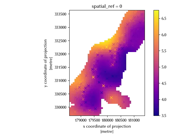
The predicted values are close enough to the observed one, so it looks like the model can be safely used in the above region.
Conclusions
Gaussian processes enable you to smoothly interpolate geostatistical data, and PyMC enables you to fully customize your model and compare the model performances.
%load_ext watermark

%watermark -n -u -v -iv -w -p xarray,pytensor,numpyro,jax,jaxlib
Python implementation: CPython
Python version : 3.12.8
IPython version : 8.31.0
xarray : 2025.1.1
pytensor: 2.30.3
numpyro : 0.16.1
jax : 0.5.0
jaxlib : 0.5.0
numpy : 2.2.6
rioxarray : 0.18.2
pymc : 5.22.0
geopandas : 1.1.1
arviz : 0.21.0
seaborn : 0.13.2
xarray : 2025.1.1
matplotlib: 3.10.1
pandas : 2.3.1
Watermark: 2.5.0