

Spatial data and models
Spatial statistics is the branch of statistics which deals with spatial data. As we have seen, there are many different types of spatial data, but one can identify three main types of spatial data:
- areal data,
- geostatistical data,
- point patterns.
In all cases, one can think about the data as generated by a stochastic process
\[\{ Z(s) : s \in D \subset \mathbb{R}^d \}\]and what differs among the data type is the domain $D$.
For areal data, the domain is a fixed countable collection of areal units, and this kind of data is generally obtained by performing some kind of aggregation at the spatial level. Examples of this kind of data is the number of hospitalized patients in one day per country.
For geostatistical data, the domain is instead a continuous subset, but we generally only perform the observations on a given set of points of this subset. Examples of geostatistical data are temperature, humidity but also terrain elevation or any other quantity defined over the entire space.
Finally, in the case of point patterns, the domain D is itself a random quantity, and examples of point patterns are the location of lightning during a day.
We will now focus on areal data, while geostatistical data and point patterns will be discussed in future posts.
Bayesian models for areal data
Models for spatial data differs from other models by the fact that they try and encode spatial correlation into the model. The simplest family of models we can use for this is the hierarchical one, which we already extensively discussed in this post, and in the simplest case, we can assume
\[y \sim 1 \vert region\]or, in other terms
\[y_i \sim \mathcal{N}(u_i, \sigma)\]where the latent variables are iid.
\[u_i \sim \mathcal{N}(\mu, \rho)\,.\]Another kind of common model is the family of Spatial Autoregressive Models (SAR)
\[y_i \sim \mathcal{MvN}(I \mu, \Sigma)\]where $I$ represents the identity matrix. In order to account for spatial correlation and to ensure positivity, $\Sigma$ is taken as
\[\Sigma = A D A^T\]where $D$ is diagonal and
\[A = (I - B)^{-1}\]The model is generally simplified by assuming
\[D = \sigma^2 I\]and
\[B = \rho W\]where the matrix W is the adjacency matrix
\[W_{ij} = \begin{cases} 1 & \text{ if } i \text{ and } j \text{ are adjacent} \\ 0 & \text{ otherwise.}\\ \end{cases}\]A more general model is the CAR model, where we assume
\[\Sigma = \bar{D} (1-B)\,.\]Also in this case $\bar{D}$ and $B$ are generally simplified by taking $B$ as above and
\[\bar{D} = \tau \text{ diag}(\sum_i W_{ij})\]Since the SAR model is a special case of the CAR one, we will neglect the first one and focus on the latter.
The Italy West Nile dataset
In this example we will use the data kindly provided by Francesco Branda in the West Nile github repo, where both human and animal known West Nile virus infections in Italy are collected for all the summer period since 2012.
We choose this dataset since, being the West Nile an infectious disease, it is reasonable to assume that spatial correlation plays a crucial role.
In our analysis we will fit the new infections reported in one week, and we will use a Poisson likelihood. As prior for the log of the Poisson mean we will both use an iid gaussian distribution and a CAR model in order to compare the performances of the two models.
import pandas as pd
import geopandas as gpd
import seaborn as sns
import pymc as pm
import arviz as az
import numpy as np
from matplotlib import pyplot as plt
import libpysal as lp

rng = np.random.default_rng(42)

year=2023

df_prov = pd.read_csv(f'https://raw.githubusercontent.com/fbranda/west-nile/main/{year}/human-surveillance/wn-ita-provinces-human-surveillance-{year}.csv')

shpfile_provs = "../geo/shape/limits_IT_provinces.geojson"

provs = gpd.read_file(shpfile_provs)

df0 = df_prov[~df_prov['new_cases'].isna()]

df0 = df0[~df0['code_province'].isna()]

df0['code_province'] = df0['code_province'].astype(int)

df0['new_cases'] = df0['new_cases'].astype(int)

df_tmp = df0.groupby(['data', 'code_province'])['new_cases'].sum().reset_index()

df_eda = pd.merge(provs, df_tmp[df_tmp['data']=='2023-08-16'], left_on='prov_istat_code_num', right_on='code_province',
                  how='left')

fig, ax = plt.subplots()
df_eda.plot('new_cases', cmap='plasma', ax=ax)
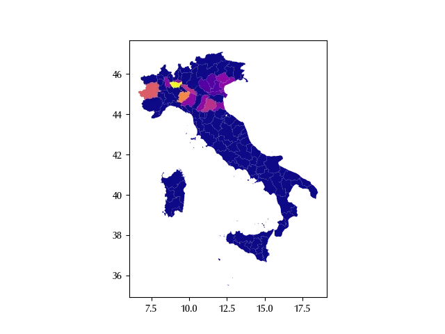
The spatial correlation looks quite evident, and this should immediately tell us that we should somehow account for it. Let us first perform a little bit more of preprocessing in order to only include the peninsular data.
df_fit = df_tmp.pivot(index='data', columns='code_province', values='new_cases').fillna(0).astype(int)

cols_incluse = range(1, 19)

provs_df = provs[provs['reg_istat_code_num'].isin(cols_incluse)].sort_values(by='prov_istat_code_num')

provs_all = provs_df['prov_istat_code_num'].values

cols_drop = [col for col in df_fit.columns if col not in provs_all]

for cd in provs_all:
    if cd not in df_fit.columns:
        df_fit[cd] = 0

df_fit_start = df_fit[[col for col in provs_all]]

df_filt = df_fit_start.loc['2023-08-16']

coords_reg = {'prov': df_filt.index}
The hierarchical model
Let us first see what happens when we include correlation, but we don’t include any kind of geographic information into our model.
with pm.Model(coords=coords_reg) as model_hr:
    tau_spat = pm.HalfCauchy("tau_spat", 1)
    rho = pm.Normal('rho', 0, 20)
    mu = pm.Normal('mu', mu=rho, sigma=tau_spat, dims=('prov'))
    exp_mu = pm.Deterministic('exp_mu', pm.math.exp(mu), dims=('prov'))
    y = pm.Poisson('y', mu=exp_mu, observed=df_filt.values, dims=('prov'))

with model_hr:
    idata_hr = pm.sample(nuts_sampler='numpyro', draws=2000, tune=2000, target_accept=0.95, random_seed=rng)

az.plot_trace(idata_hr)
fig = plt.gcf()
fig.tight_layout()
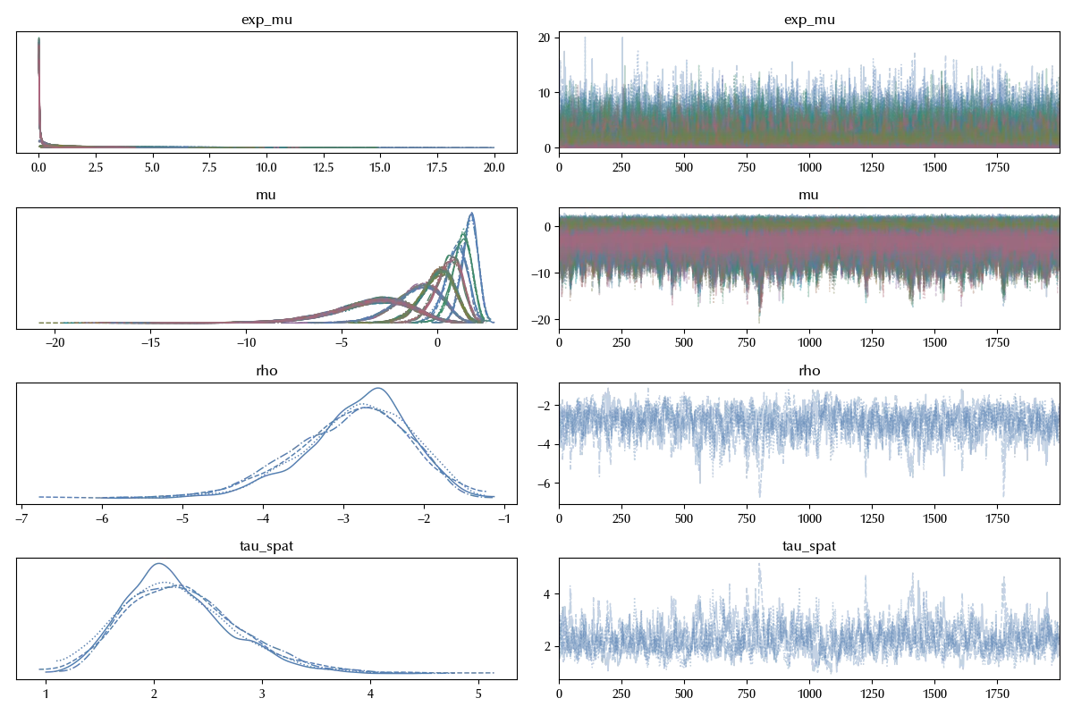
There are no sampling issue, we can now start assessing the performances of our model.
with model_hr:
    idata_hr.extend(pm.sample_posterior_predictive(idata_hr, random_seed=rng))

fig, ax = plt.subplots()
az.plot_ppc(idata_hr, ax=ax)
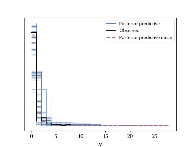
By looking at the posterior predictive distribution it’s hard to say what’s goind on, so let us try with the LOO.
with model_hr:
    pm.compute_log_likelihood(idata_hr)

fig, ax = plt.subplots()
az.plot_loo_pit(idata_hr, y='y', ax=ax)
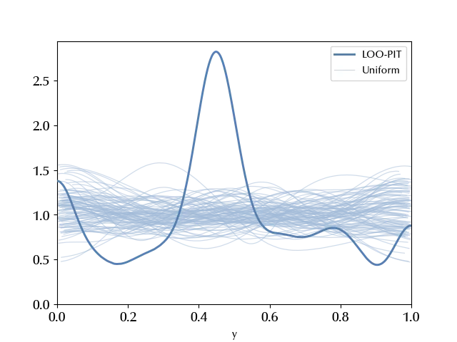
Here the situation looks way more clear, and we have an overdispersed model (recall our previous discussion about the model assessment) .
The CAR model
Let us now try and include the geographic information via the CAR model. First of all, let’s compute the adjacency matrix, and we will use libpsal to do this.
gdf_neighbors = lp.weights.Queen.from_dataframe(provs_df, use_index=False)

gdf_adj_mtx, gdf_adj_mtx_indices = gdf_neighbors.full()

with pm.Model(coords=coords_reg) as model:
    alpha = pm.Beta('alpha', alpha=1/2, beta=1/2)
    tau_spat = pm.HalfCauchy("tau_spat", 1)
    rho = pm.Normal('rho', 0, 20)
    mu = pm.CAR("mu", mu=rho*np.ones(len(df_fit_start.columns)), tau=tau_spat, alpha=alpha, W=gdf_adj_mtx, dims="prov")
    exp_mu = pm.Deterministic('exp_mu', pm.math.exp(mu), dims=('prov'))
    y = pm.Poisson('y', mu=exp_mu, observed=df_filt.values, dims=('prov'))

with model:
    idata = pm.sample(nuts_sampler='numpyro', draws=2000, tune=2000, target_accept=0.95, random_seed=rng)

az.plot_trace(idata)
fig = plt.gcf()
fig.tight_layout()
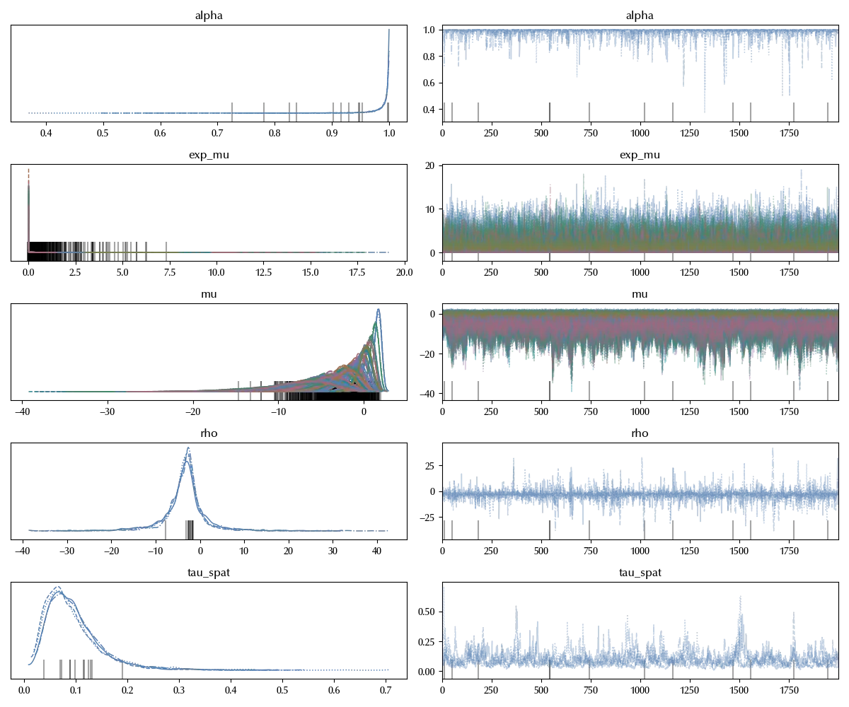
Also in this case the trace looks good. Notice that the parameter $\alpha$, which represents the spatial correlation, is very close to 1. This could lead to some issue, and in this case you could consider using an ICAR model, which is the (improper) distribution obtained by setting the correlation to 1.
with model:
    idata.extend(pm.sample_posterior_predictive(idata, random_seed=rng))

fig, ax = plt.subplots()
az.plot_ppc(idata, ax=ax)
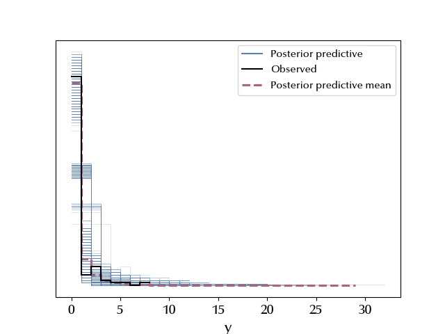
Also in this case we can’t conclude much from the PPC, so let us go with the LOO method.
with model:
    pm.compute_log_likelihood(idata)

fig, ax = plt.subplots()
az.plot_loo_pit(idata_hr, y='y', ax=ax)
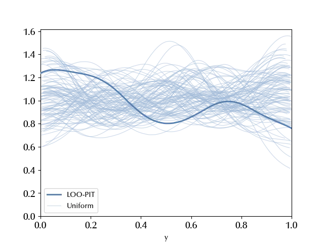
In this case the situation looks way better, let’s see if arivz confirms our feelings once taking into account the number of degrees of freedom.
df_comp = az.compare({'hierarchical': idata_hr, 'CAR': idata})

az.plot_compare(df_comp)
fig = plt.gcf()
fig.tight_layout()
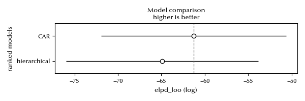
The ELPD looks better for the CAR model, and this suggests we should go for it. Let us plot the log averages for the two models on a map in order to better understand the model differences.
vmin = np.min([idata.posterior['mu'].mean(dim=('draw', 'chain')).values, idata_hr.posterior['mu'].mean(dim=('draw', 'chain')).values])
vmax = np.max([idata.posterior['mu'].mean(dim=('draw', 'chain')).values, idata_hr.posterior['mu'].mean(dim=('draw', 'chain')).values])

fig, ax = plt.subplots(ncols=2)
df_plot = provs_df.copy()
df_plot['y'] = idata_hr.posterior['mu'].mean(dim=('draw', 'chain')).values
ax[0].set_title("Hierarchical")
df_plot.plot('y', ax=ax[0], cmap='plasma', vmin=vmin, vmax=vmax)
ax[0].set_xticks([])
ax[0].set_yticks([])

df_plot1 = provs_df.copy()
df_plot1['y'] = idata.posterior['mu'].mean(dim=('draw', 'chain')).values
ax[1].set_title("CAR")
df_plot1.plot('y', ax=ax[1], cmap='plasma', vmin=vmin, vmax=vmax)
ax[1].set_xticks([])
ax[1].set_yticks([])

fig.tight_layout()
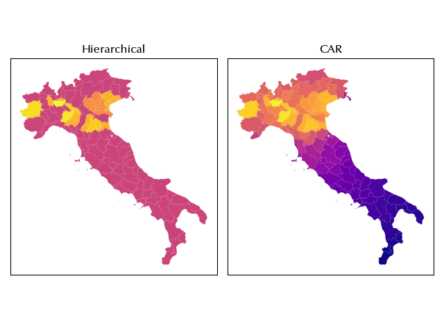
From the above figure we can see that, in the CAR model, the average smoothly decreases moving away from the observed cases. Since the hierarchical model contains no information regarding the spatial structure of the problem, the above smoothness cannot of course be observed with it.
In other terms, if you have any reason to assume that the spatial structure of the problem is relevant, you should try and include it into your model.
Conclusions
Including the spatial structure into the model can be crucial in order to fit your data, and the CAR model is a simple yet very effective way to do so for areal data.
Suggested readings
- Banerjee, S., Carlin, B. P., Gelfand, A. E. (2003). Hierarchical Modeling and Analysis for Spatial Data. Stati Uniti: CRC Press.
- Moraga, P. (2023). Spatial Statistics for Data Science: Theory and Practice with R. Regno Unito: CRC Press.
%load_ext watermark

%watermark -n -u -v -iv -w -p xarray,pytensor,numpyro,jax,jaxlib
Python implementation: CPython
Python version : 3.12.8
IPython version : 8.31.0
xarray : 2025.1.1
pytensor: 2.30.3
numpyro : 0.16.1
jax : 0.5.0
jaxlib : 0.5.0
pandas : 2.3.1
arviz : 0.21.0
pymc : 5.22.0
geopandas : 1.1.1
libpysal : 4.12.1
matplotlib: 3.10.1
numpy : 2.2.6
seaborn : 0.13.2
Watermark: 2.5.0