Hierarchical models

There are many circumstances where your data are somehow connected, but cannot be treated as iid. As an example, when you compare clinical studies on the effectiveness of a medicine, data originated from different studies will likely involve different inclusion policies as well as different hospital setup. However, it is reasonable to assume that parameters describing different studies are related.

In Bayesian statistics, a common approach in these situations is to assume that the parameters are sampled from a common prior distribution.

Mathematically speaking, you assume that

\[Y_i \sim P(\theta_i)\]

so each observation will be described by its own parameter. However, the parameters are considered as iid

\[\theta_i \sim P'(\phi)\]

This kind of model strictly belongs to the Bayesian framework, as in the frequentist one the parameters $\theta_i$ are numbers, so you can either treat them as different (unpooled) or they are sampled from the same distribution (pooled). Hierarchical models are one of the major components of the modern statistics, so it is worthwhile spending some time to deeply understand this model family.

A little digression on pooling

In statistics, pooling refers to the practice of grouping different observations assuming that they are identically distributed. In order to better explain this concept, let us assume that we have $N$ observations $y_1,y_2,\dots,y_N\,.$

In the unpooled model you assume that each observation is associated to a probability distribution, and that every distribution is independent on the other distributions. Assuming an unpooled model means associating a different parameter to each observation.

The structure of the unpooled model

In the pooled model, you assume that all the observations are associated to the same probability distribution. In this case, all the observations are related to the same parameter.

The structure of the pooled model

In the hierarchical model each observation has its own parameter, but the parameters are all sampled from the same distribution.

The structure of the hierarchical model

Let us take a look at these different kind of models with a simple example.

SpaceX analysis

In the following we will consider the launches from the four main launch vehicles: Falcon 1, Falcon 9, Falcon Heavy and Starship ¹. For the sake of simplicity, we will treat as identical rockets of different variants within the same family. Below we provide the relevant statistics for the different launchers.

	Mission	Number	successes
0	Falcon 1	5	2
1	Falcon 9	304	301
2	Falcon Heavy	9	9
3	Starship	9	5

import pandas as pd
import numpy as np
import seaborn as sns
import pymc as pm
import arviz as az
import scipy.stats as st
from matplotlib import pyplot as plt

df_spacex = pd.DataFrame({'Mission': ['Falcon 1', 'Falcon 9', 'Falcon Heavy', 'Starship'], 'N': [5, 304, 9, 9], 'y': [2, 301, 9, 5]})

df_spacex['mu'] = df_spacex['y']/df_spacex['N']

rng = np.random.default_rng(42)

coords = {'obs_id': df_spacex['Index']}

No pooling

Let us first consider the no pooling model, where we assume that the failure probability of each vehicle is independent on the other vehicles.

with pm.Model(coords=coords) as spacex_model_no_pooling:  
  theta = pm.Beta('theta', alpha=1/2, beta=1/2, dims=['obs_id'])
  y = pm.Binomial('y', p=theta, n=df_spacex['N'].values,
                  observed=df_spacex['y'].values, dims=['obs_id'])

pm.model_to_graphviz(spacex_model_no_pooling)

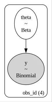
The structure of the unpooled model

In the above diagram we see that each of the four vehicle has its own parameter.

with spacex_model_no_pooling:
    idata_spacex_no_pooling = pm.sample(5000, tune=5000, chains=4,
                                        random_seed=rng, target_accept=0.95,
                                       nuts_sampler='numpyro')

az.plot_trace(idata_spacex_no_pooling)
fig = plt.gcf()
fig.tight_layout()

The trace of the unpooled model

In the above block, we increased the “target_accept” parameter in order to avoid numerical issues. The trace looks fine, but let us now take a better look at the estimated parameters.

az.plot_forest(idata_spacex_no_pooling)

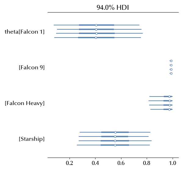
The forest plot of the unpooled model

The parameters make sense, and the Falcon 1 as well as the Starship are very unconstrained, due to the small number of launches. Let us now take a look at the pooled model.

Full pooling

On the other hand, in the full-pooling method we assume that the same probability describes all the vehicles.

with pm.Model(coords=coords) as spacex_model_full_pooling:  
  theta = pm.Beta('theta', alpha=1/2, beta=1/2)
  y = pm.Binomial('y', p=theta, n=df_spacex['N'].values,
                  observed=df_spacex['y'].values, dims=['obs_id'])

pm.model_to_graphviz(spacex_model_full_pooling)

The structure of the pooled model

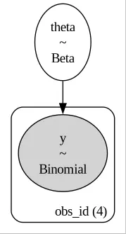
In this model, all the launches are treated as sampled from a common iid, and we therefore have only one parameter for all the launch vehicle.

with spacex_model_full_pooling:
  idata_spacex_full_pooling = pm.sample(5000, tune=5000, chains=4,
                                        random_seed=rng, target_accept=0.95,
                                       nuts_sampler='numpyro')

az.plot_trace(idata_spacex_full_pooling)
fig = plt.gcf()
fig.tight_layout()

The trace of the pooled model

az.plot_forest(idata_spacex_full_pooling)

The forest plot of the pooled model

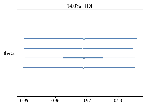
In this case the single parameter is almost entirely above 0.94, so any launch should succeed with a probability higher than the 94%. Would you to bet that a Falcon 1 would succeed? I honestly wouldn’t, but this is what you should do according to this model.

Hierarchical model

The hierarchical model has both the above models as special cases.

with pm.Model(coords=coords) as spacex_model_hierarchical:
    alpha = pm.HalfNormal("alpha", sigma=10)
    beta = pm.HalfNormal("beta", sigma=10)
    mu = pm.Deterministic("mu", alpha/(alpha+beta))
    theta = pm.Beta('theta', alpha=alpha, beta=beta, dims=['obs_id'])
    y = pm.Binomial('y', p=theta, n=df_spacex['N'].values,
                  observed=df_spacex['y'].values, dims=['obs_id'])

pm.model_to_graphviz(spacex_model_hierarchical)

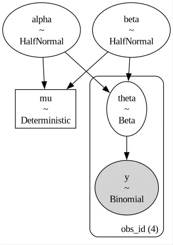
The structure of the hierarchical model

In this case, each vehicle has its own parameter. The parameters are however sampled according to a Beta distribution, with priors $\alpha$ and $\beta\,.$

with spacex_model_hierarchical:
    idata_spacex_hierarchical = pm.sample(5000, tune=5000, chains=4,
                                        random_seed=rng, target_accept=0.95,
                                       nuts_sampler='numpyro')

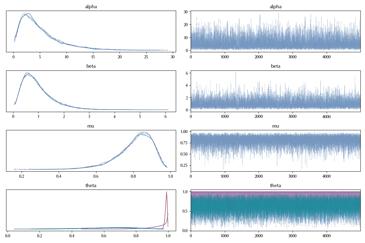
The trace of the hierarchical model

az.plot_forest(idata_spacex_hierarchical)

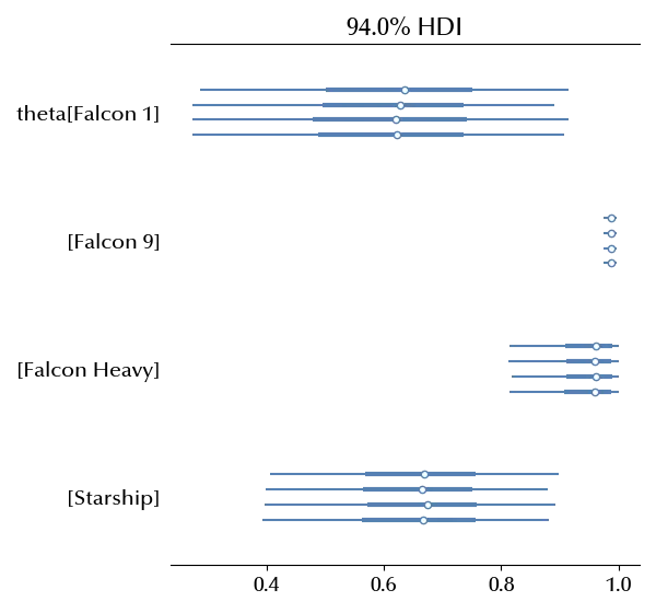
The forest plot of the hierarchical model

These estimates are similar to the unpooled model, they are however closer one to the other ones. This can be easily seen by comparing the two forest plot

fig = plt.figure()
ax = fig.add_subplot(111)
az.plot_forest([idata_spacex_no_pooling, idata_spacex_hierarchical], model_names=['no pooling', 'hierarchical'],
               var_names=['theta'], ax=ax, combined=True)
fig.tight_layout()

The forest plot of the hierarchical model compared to the unpooled model

This happens because the hierarchical model allow us to share information across the variables.

One of the most relevant features of hierarchical models, is that they allow us to make predictions for unobserved variables with unknown parameters. Let us assume that SpaceX produces a new launcher, this model allows us to estimate its success probability.

with spacex_model_hierarchical:
    theta_new = pm.Beta('th_new', alpha=alpha, beta=beta)
    ppc_new = pm.sample_posterior_predictive(idata_spacex_hierarchical, var_names=['th_new'])

az.plot_posterior(ppc_new.posterior_predictive['th_new'].values.reshape(-1))

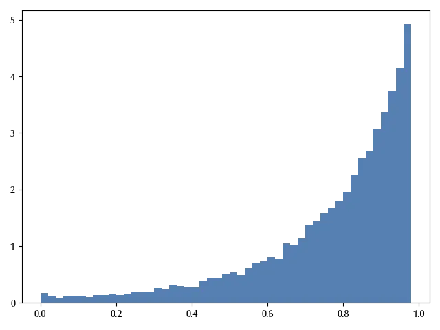
The probability distribution for a new theta

We can moreover estimate the average success rate for any SpaceX vehicle.

map_mu = st.mode(np.digitize(idata_spacex_hierarchical.posterior["mu"].values.reshape(-1), bins=np.linspace(0, 1, 100))).mode/100

fig = plt.figure()
ax = fig.add_subplot(111)
az.plot_posterior(idata_spacex_hierarchical, var_names=["mu"], ax=ax)
ax.text(0.3, 3, f'MAP: {map_mu}', fontsize=15)

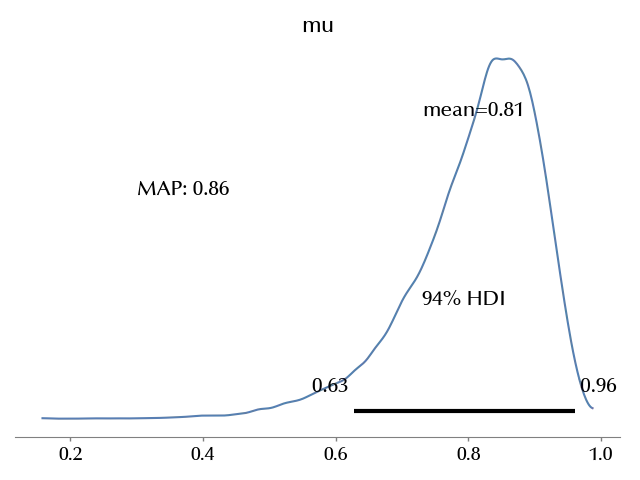
The probability distribution of a success

This estimate is much more generous than the pooled one, as it properly takes into account the failure rates of less successful models.

We also reported the Maximum A Posteriori (MAP) estimate for the above parameter, as it is a better point estimate than the mean for non-symmetric distributions as the one above.

Conclusions

We discussed how hierarchical models allow us to share information across the variables and to make predictions for new, unobserved, variables. In the next post we will discuss a very important application of hierarchical models to meta-analysis.