Hierarchical models and meta-analysis

In the last post we discussed how to build a hierarchical model. These models are often used in meta-analysis and reviews, i.e. in academic publications where the results of many studies are collected, criticized and combined. In this kind of study using a full pooling would not be appropriate, as each study is performed at its own conditions, so a hierarchical model is much more appropriate to combine the results together. This topic is extensively discussed in Gelman’s textbook, and we will limit ourselves to show an application of hierarchical model to the meta-analysis.

We will use this method to re-analyze an old meta-analysis by Daryl Bem, a well known researcher who published the famous “Bem meta-analysis” where he suggested that he found some evidence of precognition. This paper became very famous both because of the conclusions and because researchers failed to replicate its findings.

By analyzing the methodological flaws used in that paper, other scientist started proposing many methods to improve the robustness of the research results.

We won’t analyze that article, since it combined many kinds of experiments, and this makes the overall analysis more involved. We will instead use another paper by the same author which can be found on this page of the CIA website (yes, CIA has been really interested into paranormal activity). We choose this article as it simply involves a binomial likelihood. The article, in fact, summarizes the results of 11 experiments which has equi-probable binary outcome, so by random guessing one would expect, on average, a success percentage of the $50\%\,.$

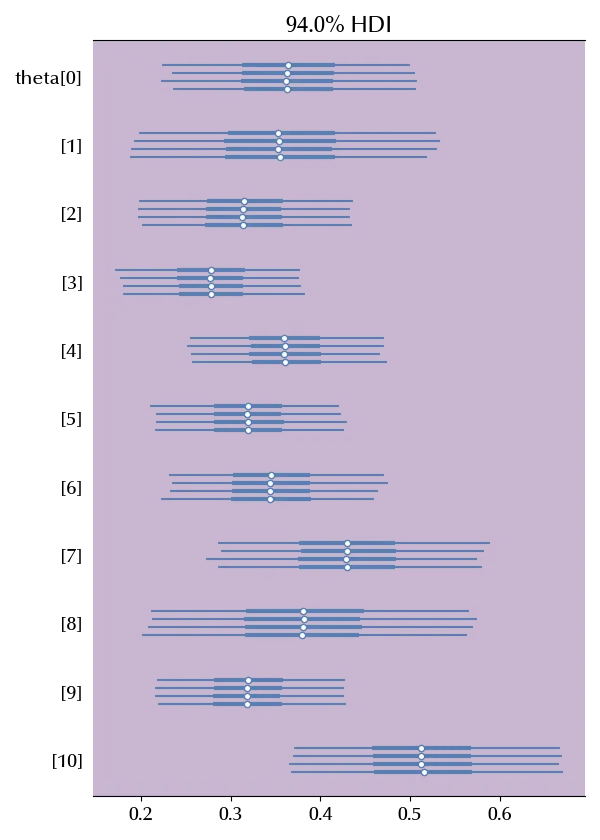
In the analysis we will use the Region Of Practical Equivalence (ROPE) to assess if the effect is practically equivalent with absent. We will conclude that there is no evidence of precognition if the $94\%$ Highest Density Region for the average success ratio is entirely included in the region $[0, 0.75]\,.$ We will instead conclude that there is evidence of precognition if the $94\%$ HDI is entirely inside the $[0.75, 1]$ region. If the $94\%$ HDI crosses 0.75 we will conclude that the analysis is inconclusive.

The limit 0.75 seems quite strong, but since a positive finding would contradict the current scientific knowledge, we require a strong evidence in order to get a positive result. Notice that the ROPE choice must be done before the dataset is seen, otherwise we could tune the choice on the data.

As before, we will take

\[\begin{align} \alpha \sim & \mathcal{HN}(10) \\ \beta \sim & \mathcal{HN}(10) \\ \theta_i \sim & \mathcal{Beta}(\alpha, \beta) \\ y_i \sim & \mathcal{Binom}(\theta_i, n_i) \end{align}\]

where $\mathcal{HN}(\sigma)$ denotes the Half Normal distribution.

Our dataset will consist into the 4th and 5th columns of table 1, which we provide here

n	y
22	8
9	3
35	10
50	12
50	18
50	15
36	12
20	10
7	3
50	15
25	16

import pandas as pd
import numpy as np
import seaborn as sns
import pymc as pm
import arviz as az
import scipy.stats as st
from matplotlib import pyplot as plt

rope_reg = [0, 0.75]

df = pd.DataFrame({"n": [22, 9, 35, 50, 50, 50, 36, 20, 7, 50, 25], 
                   "y": [8, 3, 10, 12, 18, 15, 12, 10, 3, 15, 16]})

rng = np.random.default_rng(42)

with pm.Model() as binom_meta:
    alpha = pm.HalfNormal("alpha", sigma=10)
    beta = pm.HalfNormal("beta", sigma=10)
    theta = pm.Beta('theta', alpha=alpha, beta=beta, shape=len(df['n'].values))
    y = pm.Binomial('y', p=theta, n=df['n'].values,
                  observed=df['y'].values)

with binom_meta:
    idata_meta = pm.sample(5000, tune=5000, chains=4, target_accept=0.98,
                           random_seed=rng, nuts_sampler='numpyro')

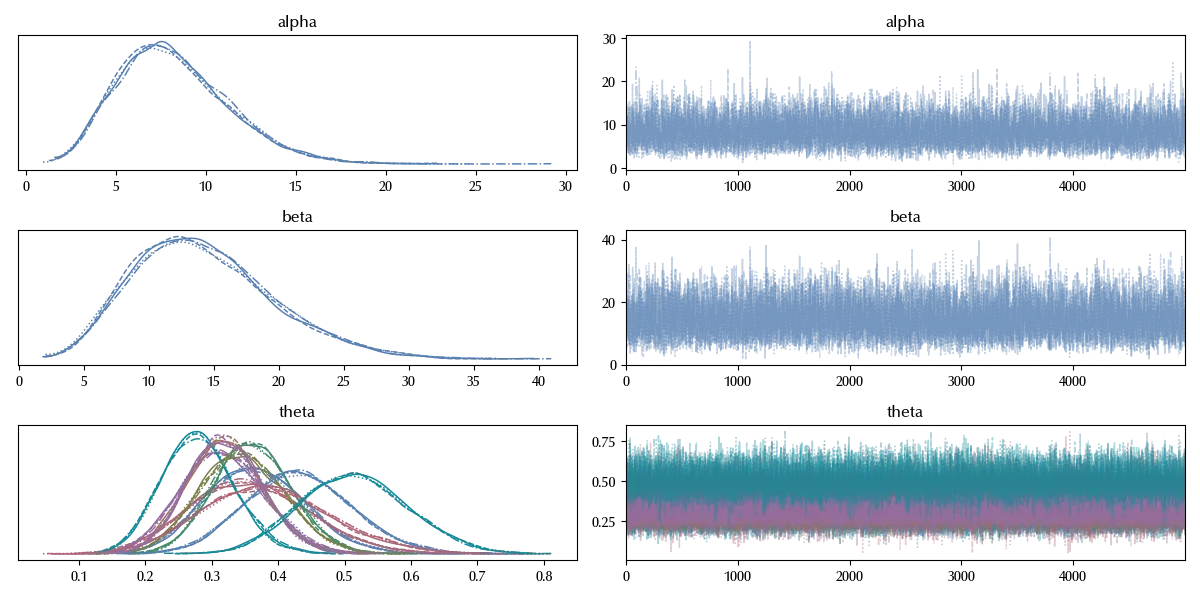
az.plot_trace(idata_meta)
fig = plt.gcf()
fig.tight_layout()

The trace of the hierarchical model

az.summary(idata_meta)

	mean	sd	hdi_3%	hdi_97%	mcse_mean	mcse_sd	ess_bulk	ess_tail	r_hat
alpha	8.234	3.079	2.857	13.904	0.03	0.021	9818	11696	1
beta	14.226	5.351	4.903	24.217	0.051	0.036	10128	10807	1
theta[0]	0.366	0.074	0.231	0.507	0	0	23085	15421	1
theta[1]	0.357	0.09	0.191	0.528	0.001	0	22702	13380	1
theta[2]	0.316	0.063	0.196	0.433	0	0	23299	13816	1
theta[3]	0.279	0.054	0.178	0.381	0	0	23776	14155	1
theta[4]	0.362	0.058	0.255	0.471	0	0	23117	14252	1
theta[5]	0.32	0.056	0.216	0.427	0	0	24735	14446	1
theta[6]	0.346	0.064	0.226	0.464	0	0	25809	14362	1
theta[7]	0.431	0.08	0.284	0.584	0.001	0	22630	14849	1
theta[8]	0.384	0.097	0.202	0.564	0.001	0	24538	13129	1
theta[9]	0.32	0.056	0.218	0.428	0	0	23604	15030	1
theta[10]	0.515	0.081	0.369	0.67	0.001	0	20264	14867	1

There is no evident issue in the sampling procedure.

az.plot_forest(idata_meta, var_names=['theta'], rope=rope_reg)

The forest plot of the hierarchical model

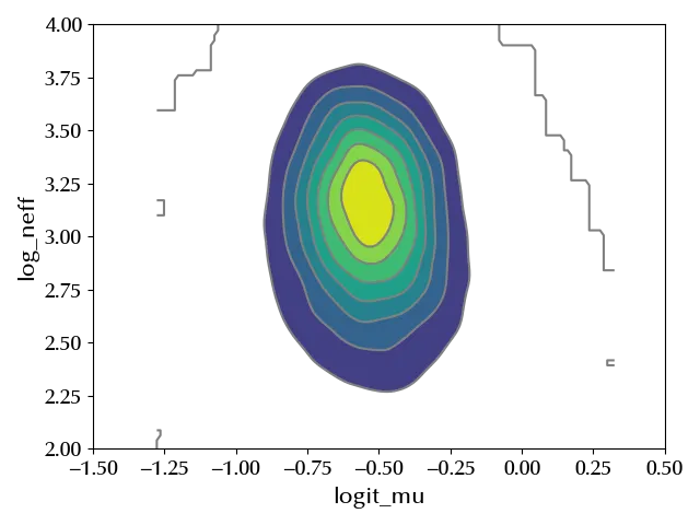
None of the studies suggests that there is any evidence of precognition. We can also estimate the overall average as well as the effective sample size.

with binom_meta:
    logit_mu = pm.Deterministic("logit_mu", pm.math.log(alpha/beta))
    log_neff = pm.Deterministic("log_neff", pm.math.log(alpha+beta))

with binom_meta:
    ppc = pm.sample_posterior_predictive(idata_meta, var_names=['logit_mu', 'log_neff'])
    
    
fig = plt.figure()
ax = fig.add_subplot(111)
az.plot_pair(ppc.posterior_predictive, var_names=["logit_mu", "log_neff"], kind="kde", ax=ax)
ax.set_xlim([-1.5, 0.5])
ax.set_ylim([2, 4])
fig.tight_layout()

The kernel density estimate for mu and for the effective sample size of the hierarchical model

Conclusions

We applied the beta binomial hierarchical model to a meta-analysis on precognition. We also introduced the Region Of Practical Equivalence (ROPE).

Conclusions

Suggested readings