Random models and mixed models

There are many situations where you want to understand the relation between two variables at the subgroup level rather than at the level of the entire sample. Random effect models are linear models where each subgroup has its own slope and intercept, while in mixed effect models you either assign a slope to each subgroup and a unique intercept or vice versa.

Let us see what are the differences between a random effect model and a fixed effect model by looking at the data of this study, where the authors restricted the number of hours of a set of participants for ten days and analyzed the reaction time of the participants to a test. The dataset only includes the set of participants who only slept for three hours per night.

import pandas as pd
import numpy as np
import jax.numpy as jnp
import seaborn as sns
from matplotlib import pyplot as plt
import pymc as pm
import arviz as az
import pymc.sampling_jax as pmj

df = pd.read_csv('data/Reaction.csv')

rng = np.random.default_rng(42)
df.head()

	Unnamed: 0	X	Reaction	Days	Subject
0	1	1	249.56	0	308
1	2	2	258.705	1	308
2	3	3	250.801	2	308
3	4	4	321.44	3	308
4	5	5	356.852	4	308

Let us normalize the data before analyzing them, and let us assume

$y_i = \alpha + \beta X_{i} + \varepsilon_i$

df['y'] = (df['Reaction'] - mean)/df['Reaction'].std()
df['subj_id']=df['Subject'].map({elem: k for k, elem in enumerate(df['Subject'].drop_duplicates())})
df['intercept'] = 1
X_v = df[['intercept','Days']]
X_s = pd.DataFrame({'subj':df['subj_id'].drop_duplicates()})
coords = {'cols': X_v.columns, 'obs_id': X_v.index, 'subj_id': X_s.index, 'subj_col': X_s.columns}


with pm.Model() as model_fixed:
    alpha = pm.Normal('alpha', mu=0, sigma=500)
    beta = pm.Normal('beta', mu=0, sigma=500)
    sigma = pm.HalfNormal('sigma', sigma=500)
    yhat = pm.Normal('y', mu=alpha + beta*df['Days'], sigma=sigma, observed=df['y'])

with model_fixed:
    idata_fixed = pm.sample(nuts_sampler='numpyro', random_seed=rng)

az.plot_trace(idata_fixed)
fig = plt.gcf()
fig.tight_layout()

yfit = jnp.outer(idata_fixed.posterior['alpha'].values.reshape(-1), jnp.ones(len(df['Days'].drop_duplicates().values)))+jnp.outer(
    idata_fixed.posterior['beta'].values.reshape(-1), jnp.arange(len(df['Days'].drop_duplicates().values)))

fig = plt.figure()
ax = fig.add_subplot(111)
ax.fill_between(df['Days'].drop_duplicates().values, jnp.quantile(yfit, q=0.03, axis=0),jnp.quantile(yfit, q=0.97, axis=0),
               color='lightgray', alpha=0.8)
ax.plot(df['Days'].drop_duplicates().values, jnp.mean(yfit, axis=0))
sns.scatterplot(df, x='Days', y='y', hue='Subject', ax=ax)
ax.get_legend().remove()
fig.tight_layout()

The estimated trend agrees with the observed one, but our model fails to reproduce the observed variability despite the large prior variance. Let us now compare the previous model with a random effect model. In this model we will assume that each individual has his/her own intercept, which represents the response without sleeping restrictions, as well as his/her own slope, which represents the average change in performance after one day of sleep restrictions. We will fully leverage bayesian statistics, and assume that the parameters have a common prior. Another possible choice would have been to assume that each of them had a separate prior, but in this way we can share information across the individuals. We will also assume that the slope and the intercept are correlated.

$\begin{align} y_i &= \alpha_{[j]i} + \beta_{[j]i} X_{i} + \varepsilon_i \\ \varepsilon_i & \sim \mathcal{N}(0, \sigma) \\ \begin{pmatrix} \alpha_{[j]i} \\ \beta_{[j]i} \end{pmatrix} & \sim \mathcal{N}(\mu, \Sigma) \\ \mu_i & \sim \mathcal{N}(0, 10) \\ \Sigma & \sim \mathcal{LKJ}(1) \end{align}$

with pm.Model(coords=coords) as model:
    mu = pm.Normal('mu', sigma=10, dims=['cols'])
    X = pm.Data('X', X_v, dims=['obs_id', 'cols'])
    sd_dist = pm.HalfNormal.dist(sigma=5, size=X_v.shape[1])
    chol, corr, sig = pm.LKJCholeskyCov('sig', n=X_v.shape[1], eta=1.0, sd_dist=sd_dist)
    sigma = pm.HalfNormal('sigma', sigma=5)
    # sig = pm.HalfNormal('sig', 5, dims=['cols'])
    alpha = pm.MvNormal(f'alpha', mu=mu, chol=chol, dims=['subj_id', 'cols'], shape=(len(df['Subject'].drop_duplicates()), X_v.shape[1]))
    tau = pm.Deterministic('tau', pm.math.sum([alpha[df['subj_id'], k]*X.T[k,:] for k in range(X_v.shape[1])], axis=0),
                          dims=['obs_id'])
    yhat = pm.Normal(f'yhat', mu=tau, sigma=sigma, observed=df['y'], dims=['obs_id'])

with model:
    idata = pm.sample(nuts_sampler='numpyro',
                     random_seed=rng)

az.plot_trace(idata, 
              coords={"sig_corr_dim_0": 0, "sig_corr_dim_1": 1})
fig = plt.gcf()
fig.tight_layout()

The trace looks fine, let us now look at the posterior predictive.

with model:
    ppc = pm.sample_posterior_predictive(idata, random_seed=rng)
    
sub_dict_inv = {k: elem for k, elem in enumerate(df['Subject'].drop_duplicates())}

x_pl = np.arange(10)
fig, ax=plt.subplots(nrows=6, ncols=3, figsize=(9, 8))
df_subs = pd.DataFrame({'Subject': df['Subject'], 
                        'Days': df['Days'],
                        'y': df['y'],
                        'mean': ppc.posterior_predictive['yhat'].mean(dim=['draw', 'chain']),
                       'low': ppc.posterior_predictive['yhat'].quantile(q=0.03, dim=['draw', 'chain']),
                       'high': ppc.posterior_predictive['yhat'].quantile(q=0.97, dim=['draw', 'chain']),
})
for i in range(6):
    for j in range(3):
        k =3*i + j
        df_red = df_subs[df_subs['Subject']==sub_dict_inv[k]]
        y_pl = df_red['mean']
        y_m = df_red['low']
        y_M = df_red['high']
        ax[i][j].fill_between(x_pl, y_m, y_M, alpha=0.8, color='lightgray')
        ax[i][j].plot(x_pl, y_pl)
        ax[i][j].scatter(df_red['Days'], df_red['y'])
        ax[i][j].set_ylim(-4, 4)
        ax[i][j].set_title(f"i={k}")
        ax[i][j].set_yticks([-4, 0, 4])
fig.tight_layout()

The performances of the new model are way better than the previous one, and this is not surprising since we have many more parameters.

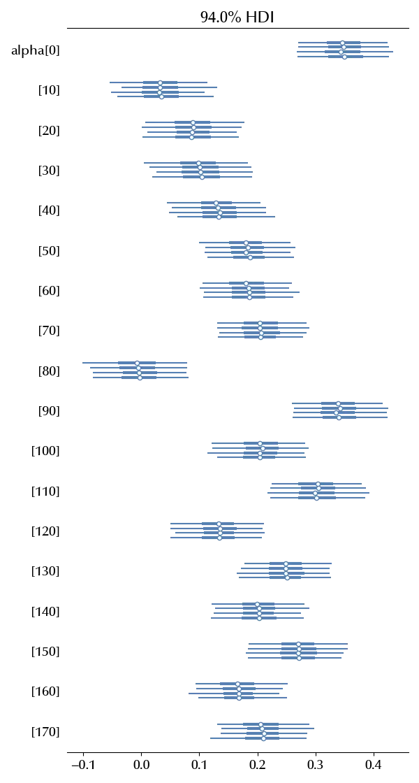
We can now verify how much does the average performance degradation changes with the participant.

az.plot_forest(idata, var_names="alpha",
              coords={"cols": ["Days"]})

We can also predict how will a new participant perform

with model:
    alpha_new = pm.MvNormal('alpha_new', mu=mu, chol=chol, shape=(2), dims=['cols'])
    tau_new = pm.Deterministic('tau_new', alpha_new[0]+alpha_new[1]*df['Days'].drop_duplicates())
    y_new = pm.Normal(f'yhat_new', mu=tau_new, sigma=sigma)

with model:
    ppc_new = pm.sample_posterior_predictive(idata, var_names=['yhat_new', 'alpha_new', 'tau_new'])

fig = plt.figure()
ax = fig.add_subplot(111)

y_pl = ppc_new.posterior_predictive[f'yhat_new'].mean(dim=['draw', 'chain'])
y_m = ppc_new.posterior_predictive[f'yhat_new'].quantile(q=0.025, dim=['draw', 'chain'])
y_M = ppc_new.posterior_predictive[f'yhat_new'].quantile(q=0.975, dim=['draw', 'chain'])
ax.plot(np.arange(10), y_pl)
ax.fill_between(np.arange(10), y_m, y_M, color='lightgray', alpha=0.8)

Another advantage of the hierarchical model is that we can estimate the distribution of the slope and intercept for a new participant

az.plot_pair(ppc_new, group='posterior_predictive', var_names=['alpha_new'], kind='kde')
fig = plt.gcf()
fig.tight_layout()

Conclusions

We discussed the main features of random models, and we discussed when it may be appropriate to use them. We have also seen what are the advantages of implementing a hierarchical structure on random effect models.

Conclusions

Suggested readings