
Leveraging mixed-effect models
In the last post we introduced multilevel models, in this post we will dig deeper and try and use them at their best. They are really powerful tools, but as usual from a great power comes great responsibility. We will also see how to use Bambi to easily implement them.
Introduction to Bambi
Building mixed-effects models can become quite messy as soon as the number of variables grows, but fortunately Bambi can help us. I am generally skeptical when it comes to use interfaces to do stuff, since I prefer having the full control of the underlying model. Bambi is however powerful enough to give us a lot of freedom in implementing the model.
Let us start by taking a look at the pointless dataset from the LME4 R library, as explained in this very nice introduction by Bodo Winter.
import pandas as pd
import seaborn as sns
import numpy as np
import pymc as pm
import arviz as az
import bambi as bmb
from matplotlib import pyplot as plt

rng = np.random.default_rng(42)

kwargs = {'nuts_sampler': 'numpyro', 'random_seed': rng,
          'draws': 2000, 'tune': 2000, 'chains': 4,
          'target_accept': 0.95}

df = pd.read_csv('http://www.bodowinter.com/tutorial/politeness_data.csv')

df.head()
| subject | gender | scenario | attitude | frequency | |
|---|---|---|---|---|---|
| 0 | F1 | F | 1 | pol | 213.3 |
| 1 | F1 | F | 1 | inf | 204.5 |
| 2 | F1 | F | 2 | pol | 285.1 |
| 3 | F1 | F | 2 | inf | 259.7 |
| 4 | F1 | F | 3 | pol | 203.9 |
As extensively described in this preprint, the dataset measures the frequency of different individuals, both males and females, with different attitudes (polite) and in different scenarios. The aim of the study is to determine the dependence of the frequency on the attitude.
Before starting, let us clean the dataset.
df.isna().any()
gender False
scenario False
attitude False
frequency True
dtype: bool
df_clean = df.dropna(axis=0)


fig, ax = plt.subplots()
sns.violinplot(df_clean, y='frequency', hue='gender', ax=ax)
fig.tight_layout()
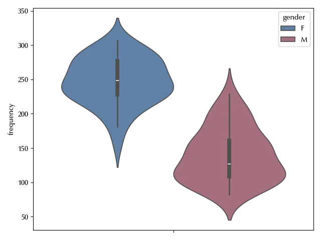
It is not surprising that the frequency depends on the gender, but it might also depend on the individual as well as on the context.
Using Bambi to fit linear models
All of our independent variables are categorical, and we will specify this to Bambi.
With Bambi you must pass a model as follows
\[y \sim model\]where mode is a string where the dependence on each variable is specified.
categoricals = ['subject', 'gender', 'scenario', 'attitude']

model_start = bmb.Model('frequency ~ gender + attitude',
                        data=df_clean, categorical=categoricals)

model_start
Family: gaussian
Link: mu = identity
Observations: 83
Priors:
target = mu
Common-level effects
Intercept ~ Normal(mu: 193.5819, sigma: 279.8369)
gender ~ Normal(mu: 0.0, sigma: 325.7469)
attitude ~ Normal(mu: 0.0, sigma: 325.7469)
Auxiliary parameters
sigma ~ HalfStudentT(nu: 4.0, sigma: 65.1447)
------
* To see a plot of the priors call the .plot_priors() method.
* To see a summary or plot of the posterior pass the object returned by .fit() to az.summary() or az.plot_trace()
We can now fit our model as follows.
idata_start = model_start.fit(**kwargs)

az.plot_trace(idata_start)
fig = plt.gcf()
fig.tight_layout()
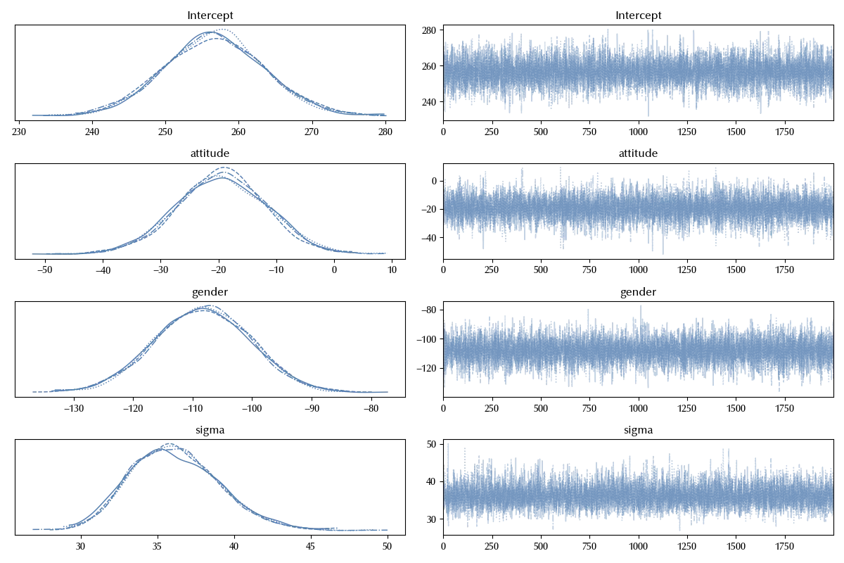
The result of the fit method is simply the inference data, exactly as the one returned by the sample method in PyMC, and the arguments of the fit method are also the arguments of the PyMC sample method.
Once you run the fit, you can also access the PyMC model by using the backend method:
pm.model_to_graphviz(model_start.backend.model)
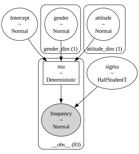
The above model for the frequency is equivalent to
\[y = \alpha + \beta_g X_g + \beta_a X_a\]where $X_g$ and $X_a$ are the indicator functions, and the priors are specified in the above model.
The intercept is automatically included, but can be explicitly included in the model with the $1$ variable as follows.
\[frequency \sim 1 + gender + attitude\]We can also remove the intercept with the $0$ variable. In this way, the first level of the first variable is not dropped. In other words, the regression variable without the $0$ is the same as
X_g = pd.get_dummies(df_clean['gender'], drop_first=True)
while with the $0$ the model becomes
\[frequency \sim 0 + gender + attitude\]which is equivalent to
\[y = \beta_g X_g + \beta_a X_a\]where this time
X_g = pd.get_dummies(df_clean['gender'], drop_first=False)
The degrees of freedom of the two models are the same, but they are differently distributed.
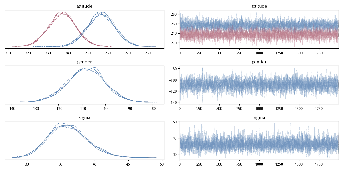
model_factor_explicit = bmb.Model('frequency ~  0  + attitude + gender',
                                  data=df_clean, categorical=categoricals)

idata_factor_explicit = model_factor_explicit.fit(**kwargs)

az.plot_trace(idata_factor_explicit)
fig = plt.gcf()
fig.tight_layout()
We can easily add an interaction term. The first way to do so is as follows
\[frequency \sim gender + attitude + gender : attitude\]A shorter notation to include the full interaction
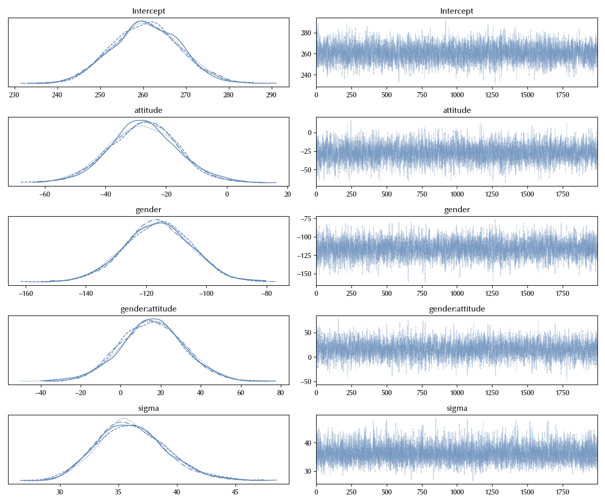
\[frequency \sim gender * attitude\]model_int = bmb.Model('frequency ~ gender * attitude',
data=df_clean, categorical=categoricals)
idata_int = model_int.fit(**kwargs)
az.plot_trace(idata_int)
fig = plt.gcf()
fig.tight_layout()
How to specify a mixed-effects model
In Bambi, one can specify the grouping by using the pipe operator. As an example, our first model with an additional subject-level random intercept can be written as
\[frequency \sim gender + attitude + (1 | subject)\]model_random_intercept = bmb.Model('frequency ~ gender + attitude + (1 | subject)',
data=df_clean, categorical=categoricals)
idata_ri = model_random_intercept.fit(**kwargs)
az.plot_trace(idata_ri)
fig = plt.gcf()
fig.tight_layout()
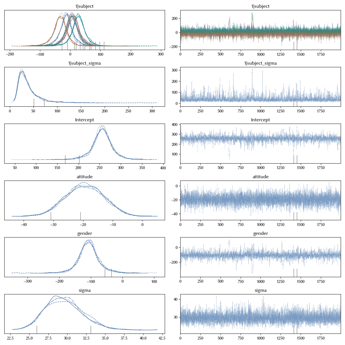
In the above model, we are allowing for the base frequency do be subject-dependence, but we are not allowing for the context dependence to do so. This does not seem logical, we should therefore include a random slope too, and we can do this as follows
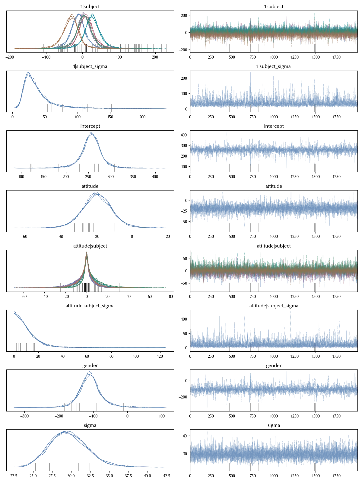
\[frequency \sim gender + attitude + (1 | subject) + (attitude | subject)\]As we have previously seen, the intercept is automatically included by Bambi once the variable is specified, and this is true for the random factors. The above model can be simplified as
\[frequency \sim gender + attitude + (attitude | subject)\]model_random_intercept_and_slope = bmb.Model('frequency ~ gender + attitude + (attitude | subject)',
data=df_clean, categorical=categoricals)
idata_rias = model_random_intercept_and_slope.fit(**kwargs)
az.plot_trace(idata_rias)
fig = plt.gcf()
fig.tight_layout()
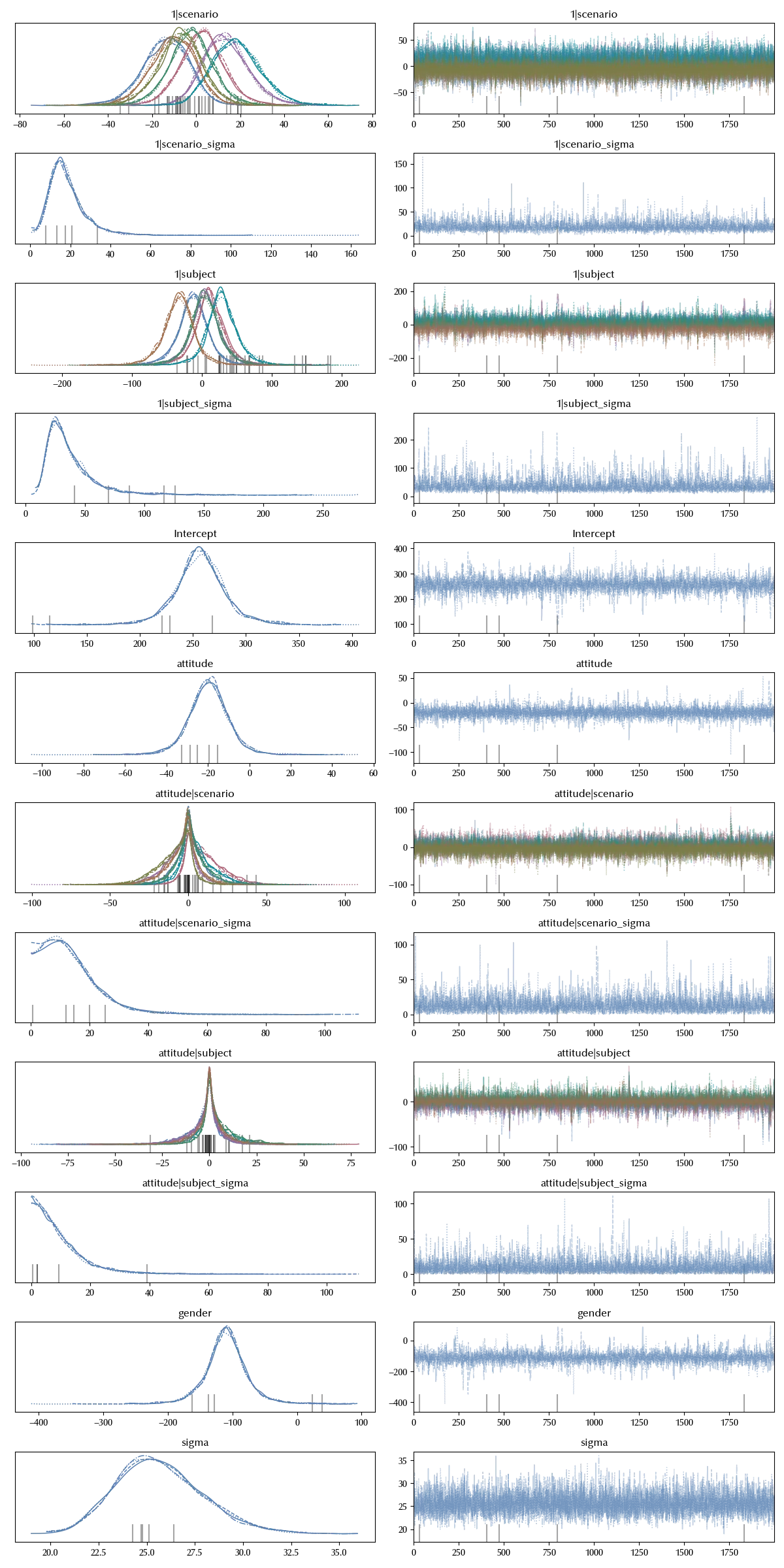
We can immediately generalize to more than one grouping factor. Let us assume we also want to quantify the scenario-dependent part of the data, we can do this as
\[frequency ~ gender + attitude + (attitude | subject) + (attitude | scenario)\]model_scenario = bmb.Model('frequency ~ gender + attitude + (attitude | subject) + (attitude | scenario)',
data=df_clean, categorical=categoricals)
idata_scenario = model_scenario.fit(**kwargs)
az.plot_trace(idata_scenario)
fig = plt.gcf()
fig.tight_layout()
Choosing a good model
We have seen that implementing a mixed-effects model in Bambi is straightforward. Since we have so much freedom, it doesn’t look easy to choose which model we should implement. Which factors should be included as random and which ones should be modelled as fixed?
Let us first ask ourselves what is a random factor, and the answer directly comes from our theory. The levels of a random factor has not been fixed in the phase of data collection, but they have been sampled from a larger population.
If we consider our dataset, we have that we have infinitely many possible scenarios, and only tree of them have been studied in our experiment. The same is true for the attitude: in the experiment the researcher asked the participants to try and stick to two attitudes, but it doesn’t make much sense to say that one can speak with only two attitudes. One can in fact experience a great variety of emotions, and express all of them when he is speaking.
Things are more tricky when we speak about the gender, since in our context we might be both be interested in the gender and, probably even more, in the biological sex. It makes in fact a lot of sense to imagine that there is a genetic component in the frequency of our voice, so we might consider replacing the gender with the sex. I personally cannot easily think about the sex of a person as sampled from a larger population. 1
By the above considerations, I might consider more appropriate to model the gender column of our dataset as a fixed factor, while in my opinion attitude and scenario are more appropriately modeled as random factors.
That said, which level of randomness should we allow in our model? There is quite a general agreement that we should allow for the largest possible level of randomness our data allows for. Half of Gelman’s textbook has been devoted to answer to this question, so I strongly recommend you to take a look it. Another interesting reading is Barr’s article where the authors analyze the effect of random factors in the context of hypothesis testing. In both cases, the answer is that if it makes sense to include a random factor, you should do so. Generally, if you allow for random slopes, you should also consider using random intercepts, and if it makes sense to include them, you should do so.
There are of course circumstances where it doesn’t make sense to do so. As an example, a pre-post experiment where the pre-test condition is fixed but the post-test is random might be modelled as a fixed-intercept random-slope.
Conclusions
Mixed-effect models can be a powerful tool for a data scientist, and Bambi can be powerful too when it comes to implement them. We have seen some of the main features of Bambi, and we briefly discussed what degree of randomness one should allow for in a mixed-effect model.
%load_ext watermark

%watermark -n -u -v -iv -w -p xarray,pytensor,numpyro,jax,jaxlib
Python implementation: CPython
Python version : 3.12.8
IPython version : 8.31.0
xarray : 2024.11.0
pytensor: 2.26.4
numpyro : 0.16.1
jax : 0.4.38
jaxlib : 0.4.38
pymc : 5.19.1
arviz : 0.20.0
seaborn : 0.13.2
numpy : 1.26.4
bambi : 0.15.0
pandas : 2.2.3
matplotlib: 3.10.0
Watermark: 2.5.0
-
Please consider this as an illustrative example, do not consider this as an opinion in psycholinguistics, as I am not an expert in this field. ↩