Mixed effects models with more than two levels

In some situations two levels are not enough do describe the data we are interested in, and here we will explain how to include them in a mixed effects model. Three-level models become popular in the context of studies on schools, since in this kind of situation there are at least three levels of interest: the student, the class and the school. It is in fact reasonable to assume that if we randomly sample two students from the same class, they will have a higher chance of being more similar in many aspects than two students coming from different classes. The same kind of consideration holds if we imagine to sample two classes from the same school and from two different schools.

In this post we will analyze the TVSFP dataset which is a subset of a dataset of a study performed to determine the efficacy of a school-based smoking prevention curriculum.

import pandas as pd
import numpy as np
import pymc as pm
import bambi as bmb
import arviz as az
import seaborn as sns
from matplotlib import pyplot as plt

rng = np.random.default_rng(42)

kwargs = {'nuts_sampler': 'numpyro', 'random_seed': rng,
          'draws': 5000, 'tune': 5000, 'chains': 4, 'target_accept': 0.9,
          'idata_kwargs': dict(log_likelihood = True)}

df = pd.read_stata('/home/stippe/Downloads/tvsfp.dta')

df['sid'] = df['sid'].astype(int)  # school id
df['cid'] = df['cid'].astype(int)  # class id
df['curriculum'] = df['curriculum'].astype(int)
df['tvprevent'] = df['tvprevent'].astype(int)

df['pid'] = range(len(df))  # pupil id

df.head()

	sid	cid	curriculum	tvprevent	prescore	postscore	pid
0	403	403101	1	0	2	3	0
1	403	403101	1	0	4	4	1
2	403	403101	1	0	4	3	2
3	403	403101	1	0	3	4	3
4	403	403101	1	0	3	4	4

Each pupil has a unique pid, each class has a unique cid and each school has a unique sid, so we don’t have to worry about non-unique labels. There are two binary variables, tvprevent and curriculum (which are the treatment factors) and two numeric (which we will consider as real, even if they are not) variables, postscore (which will be our outcome) and prescore, which is the score before the treatment. We will use all the variables to construct a linear model, and we will include an interaction term between the two treatment factors. First of all, let us try and fit the data without any hierarchical structure.

model = bmb.Model('postscore ~ prescore + tvprevent*curriculum', data=df)
idata = model.fit(**kwargs)

az.plot_trace(idata)
fig = plt.gcf()
fig.tight_layout()

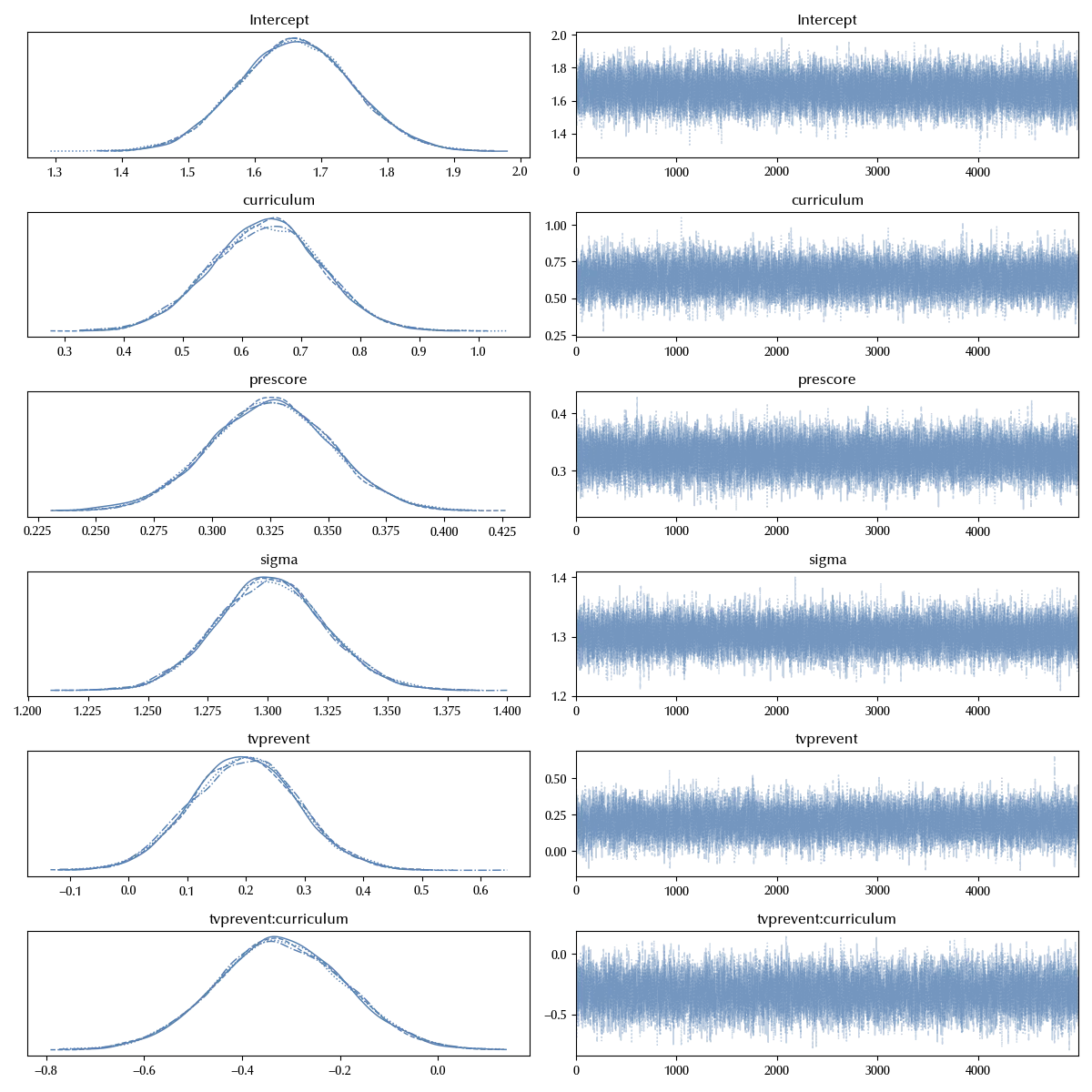
We will use this model as a baseline, adding more and more structure and comparing the results of more complex models with simpler ones, keeping the complexity level at the minimum required.

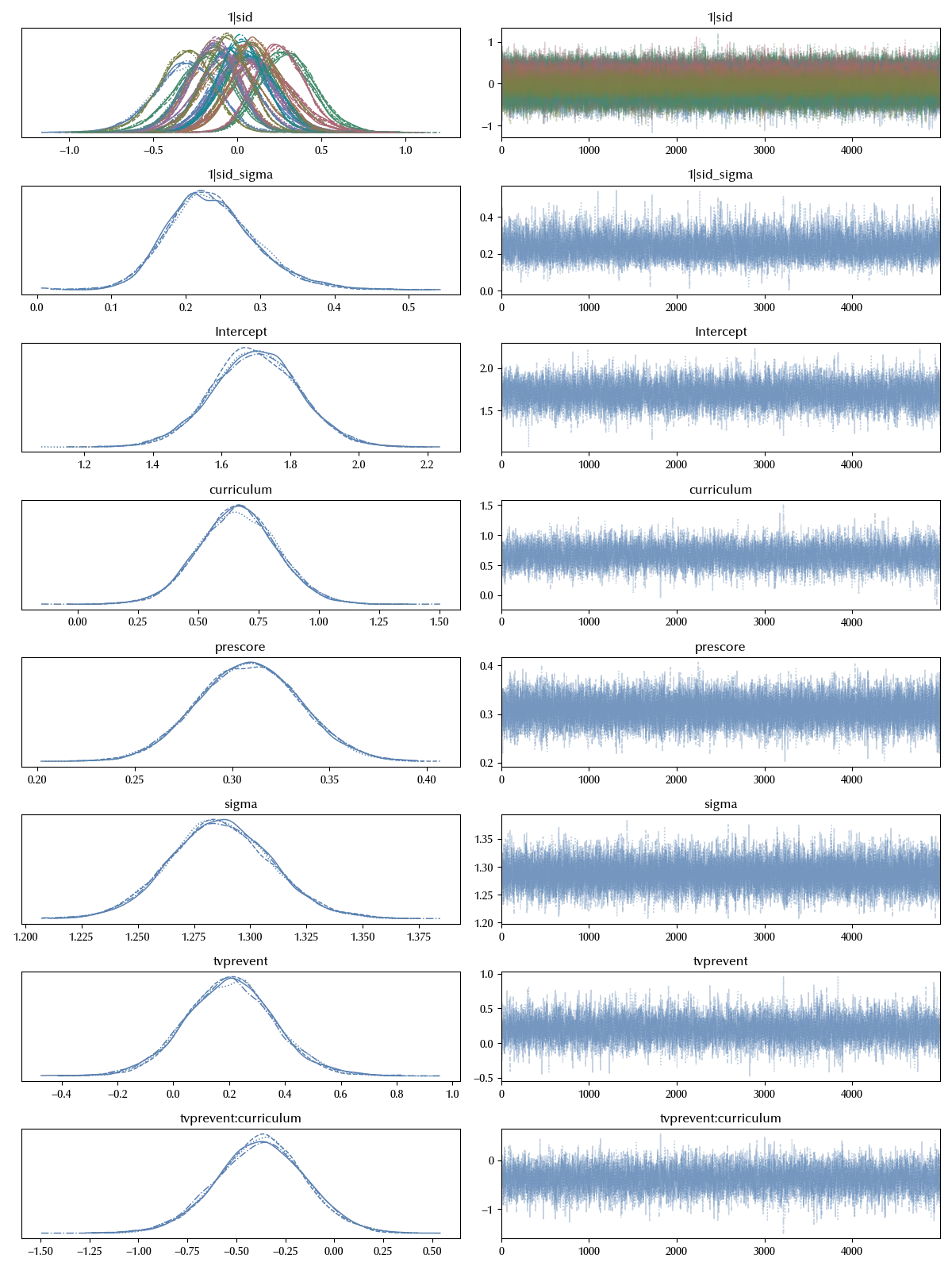
We will start by adding a school level random intercept

model_school = bmb.Model('postscore ~ prescore + tvprevent*curriculum + (1|sid)', data=df)
idata_school = model_school.fit(**kwargs)
az.plot_trace(idata_school)
fig = plt.gcf()
fig.tight_layout()

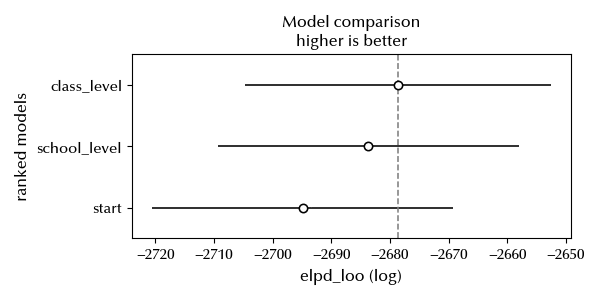
In order to compare the models we will perform a LOO ELPD estimate

df_cs = az.compare({'start': idata, 'school_level': idata_school})
az.plot_compare(df_cs)
fig = plt.gcf()
fig.tight_layout()

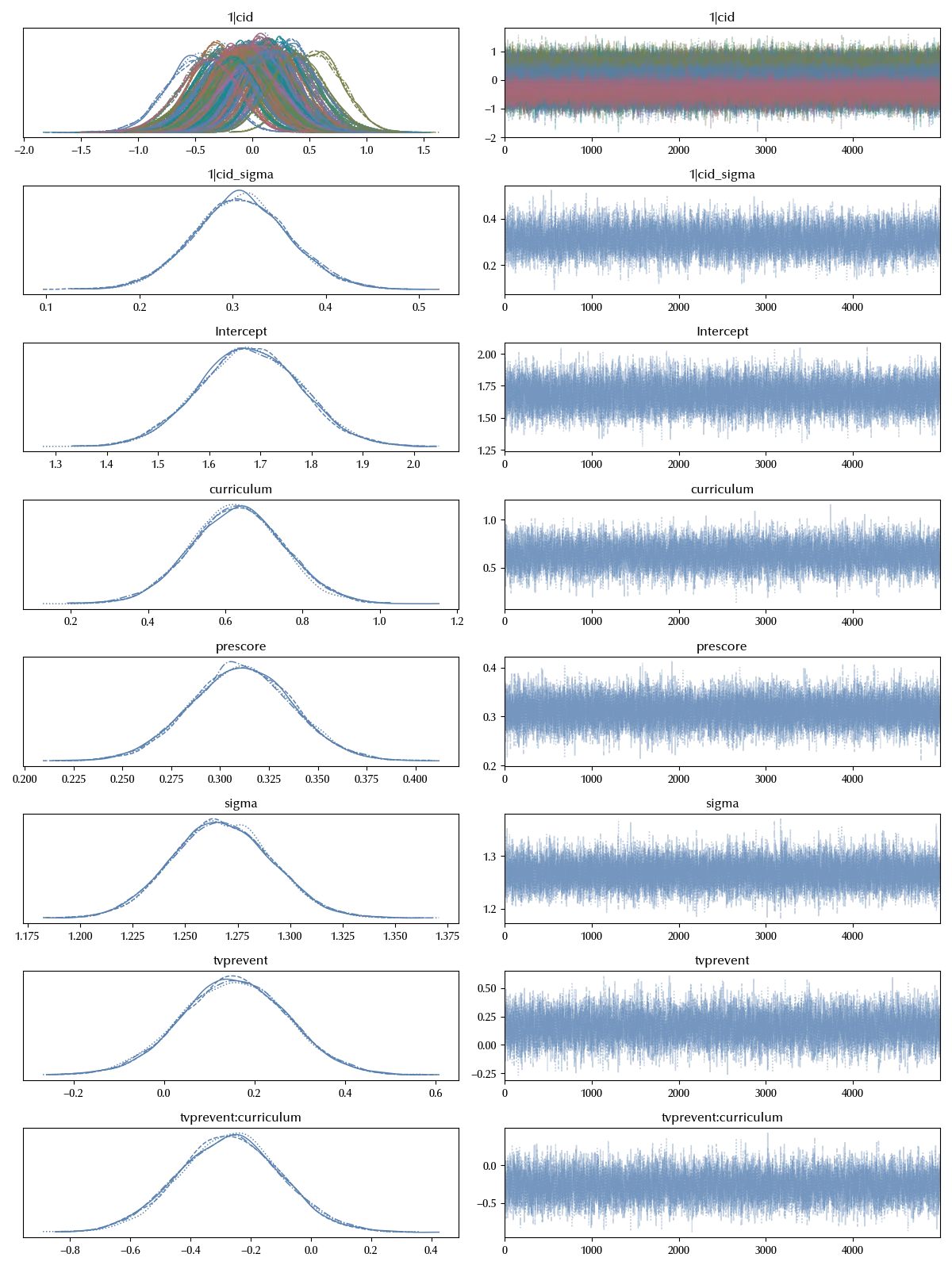
The second model seems more appropriate than the plain one, so including the school level term seems appropriate. Let us try and see what happens when we include the class level only.

model_class = bmb.Model('postscore ~ prescore + tvprevent*curriculum + (1|cid)', data=df)
idata_class = model_class.fit(**kwargs)
az.plot_trace(idata_class)
fig = plt.gcf()
fig.tight_layout()

df_csc = az.compare({'start': idata, 'school_level': idata_school, 'class_level': idata_class})
az.plot_compare(df_csc)
fig = plt.gcf()
fig.tight_layout()

Adding the class level term seems to improve even more the model. We will now try and add both of them.

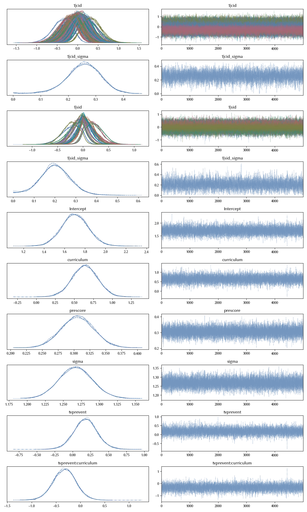
model_sc = bmb.Model('postscore ~ prescore + tvprevent*curriculum + (1|cid) + (1|sid)', data=df)
idata_sc = model_sc.fit(**kwargs)
az.plot_trace(idata_sc)
fig = plt.gcf()
fig.tight_layout()

df_csccomb = az.compare({'start': idata, 'school_level': idata_school, 'class_level': idata_class, 'school_class': idata_sc})
az.plot_compare(df_csccomb)
fig = plt.gcf()
fig.tight_layout()

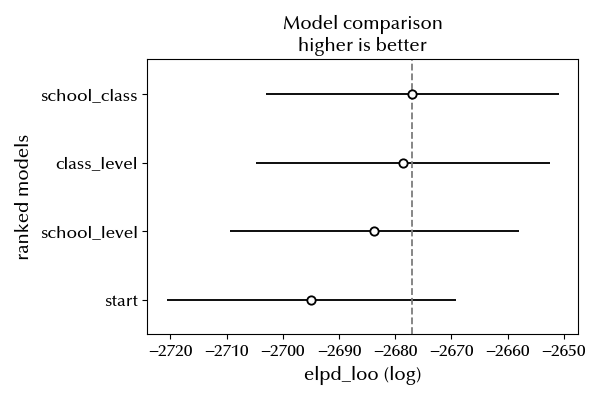
The three-levels models seems an improvement with respect to both the two-levels models, so we should stick to it when drawing conclusions about our dataset.

Conclusions

We discuss how to implement multi-level hierarchies as well as how to choose among different mixed-effects models.