

Sampling points in space
While the last time we discussed how to select points from a geodataframe, this time we will see few methods to sample random points with the only constraint of the boundaries of the region of space where the point can belong.
You can find a more in-depth discussion about this topic on Dick Brus’ page, where I found a great introduction to this topic and a properly selected bibliography as well.
Sampling methods
As you can imagine, there are different sampling strategies you can choose depending on your needs. Let us start with the more traditional ones
Grid
Grid sampling is of course the simplest method you can choose, since there is no need to perform any random sampling. There are many possible geometries, but the two most popular ones are by far the square lattice and the hexagonal lattice. Grid sampling ensures a good spatial coverage, but of course there is no randomness at all, so you might miss some relevant piece of information.
SRS
On the opposite part of the spectrum we have total randomness, and in this case we sample points from our region of interest with uniform probability. In this case coverage is only statistically ensured, while it is not guaranteed at the single sample level.
Latin hypercube sampling
We already discussed latin square sampling in the context of DoE. Latin hypercube is inspired by the above method, and it only applies to squared/rectancular raster datasets. With this method, we first divide our raster grid into a $n\times n$ grid, we then sample $n$ sub-squares according to the latin square method, and we finally sample one point from each sub-square with uniform probability.
Spatial coverage sampling
Spatial coverage sampling combines randomness with spatial coverage, and this method leverages machine learning to ensure spatial randomness. This algorithm, given an input raster, works as follows:
- We randomly choose $n$ points from our region.
- To each point of the raster, we associate the nearest point in the sample, and we clusterize our raster in this way
- we compute the centroid of the points for each cluster, and if they match with the sampled points, we stop, otherwise we replace our sample points with the new centroids, and we repeat the previous step.
Equidistant sampling
One of the most common tasks in spatial statistics is to understand the dependence of a process on the distance, and in this case none of the above method is particular effective, since either we have a totally random distance between points, or we have a very limited set of distances and directions in our sample. In this case we might prefer using equidistant sampling, where we sample points with fixed distance from a given point already present in the sample, but with random angle. Also in this case, points falling outside from the area of interested are discarded, and in this case re-sampling is performed to ensure a fixed sample size.
Python implementation
Some of the above methods require a raster dataset, other require a vector one, so we will first create both of them (in the same CRS).
import pandas as pd
import numpy as np
import geopandas as gpd
import seaborn as sns
import rasterio.plot
import matplotlib as mpl
from matplotlib import pyplot as plt
from scipy.spatial import distance
from sampling_tille import sample_square_grid, sample_hex_grid, sample_uniform_points, spatial_coverage_sampling, draw_equidistant_points
from sampling_tille.load_data import load_raster, load_data

import warnings

warnings.simplefilter("ignore")

rng = np.random.default_rng(42)

ds = load_raster('Piedmont')

gdf0 = load_data('Italy').to_crs(ds.rio.crs)

gdf = gdf0[gdf0['reg_name']=='Piemonte']

geom=gdf.to_crs(ds.spatial_ref.crs_wkt).dissolve()

fig = plt.figure(figsize=(6, 6))
ax = fig.add_subplot(111)
ds.plot(cmap=cmap,norm=norm, ax=ax)
geom.boundary.plot(ax=ax, color='k')
fig.tight_layout()
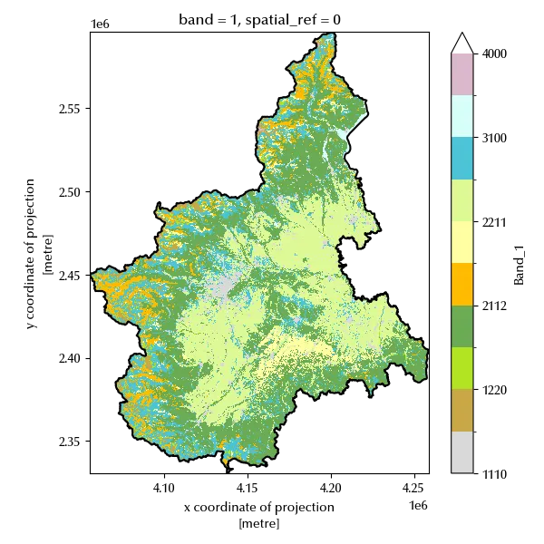
The two dataset match, as the black line corresponds to the boundaries of the geodataframe while the colored part is the altitude data contained in the raster dataset. We can now perform the sampling with the above methods. We will first compare the first four sampling method, since the last one deserves a separate treatment as it’s designed for a specific purpose.
gdf_square = sample_square_grid(geom, num_points=20)

gdf_hex = sample_hex_grid(geom, num_points=20)

gdf_unif = sample_uniform_points(geom, num_points=20, rng=rng)

# We must do a little bit more of work for the raster dataset

Xmat =np.argwhere(ds.values<65535).T
xv, yv = ds.x[Xmat[2]].values, ds.y[Xmat[1]].values

Xf = spatial_coverage_sampling(num_strata=10, xv=xv, yv=yv, rng=rng, tol=5e-2)

g0 = gpd.GeoDataFrame(geometry=gpd.points_from_xy(Xf.T[0], Xf.T[1]), crs=geom.crs)

gtmp0 = gpd.GeoDataFrame(geometry=[geom.geometry.iloc[0]]*len(gdf_square), crs=g0.crs)
gtmp1 = gpd.GeoDataFrame(geometry=[geom.geometry.iloc[0]]*len(gdf_hex), crs=g0.crs)
gtmp2 = gpd.GeoDataFrame(geometry=[geom.geometry.iloc[0]]*len(gdf_unif), crs=g0.crs)
gtmp3 = gpd.GeoDataFrame(geometry=[geom.geometry.iloc[0]]*len(g0), crs=g0.crs)

fig, ax = plt.subplots(ncols=4, sharex=True, sharey=True, figsize=(12, 5))

#geom.plot(ax=ax[0])
gtmp0.intersection(gdf_square.voronoi_polygons()).plot(ax=ax[0])
gdf_square.plot(ax=ax[0], marker='x', color='k')

gtmp1.intersection(gdf_hex.voronoi_polygons()).plot(ax=ax[1])
gdf_hex.plot(ax=ax[1], marker='x', color='k')

gtmp2.intersection(gdf_unif.voronoi_polygons()).plot(ax=ax[2])
gdf_unif.plot(ax=ax[2], marker='x', color='k')

gtmp3.intersection(g0.voronoi_polygons()).plot(ax=ax[3])

ax[3].scatter(Xf.T[0], Xf.T[1], color="k", marker="x")
ax[0].set_xlim([0.995*geom.bounds.minx.values[0], 1.005*geom.bounds.maxx.values[0]])
ax[0].set_ylim([0.995*geom.bounds.miny.values[0], 1.005*geom.bounds.maxy.values[0]])

ax[0].set_title('Square grid')
ax[1].set_title('Hex grid')
ax[2].set_title('Uniform probability')
ax[3].set_title('Spatial coverage')

fig.tight_layout()
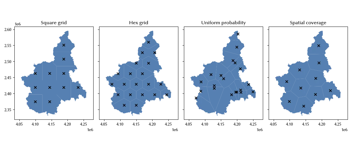
The uniform random sampling has a very poor spatial coverage, while the other methods ensure a good spatial coverage, and this is why simple random sampling is rarely used in spatial statistics.
Let us also see how to use latin hypercube sampling. For this method we must select a different dataset, since we can only use it for rectangular grids.
xds_red = load_raster("altitude")

out = sample_latin_hypercube(
    xmin=xds_red.x.min().values,
    xmax=xds_red.x.max().values,
    ymin=xds_red.y.min().values,
    ymax=xds_red.y.max().values,
    n=6,
    rng=rng,
)

fig, ax = plt.subplots()
xds_red.plot(ax=ax)
ax.scatter(out.T[0], out.T[1], marker='x', c='r')
fig.tight_layout()
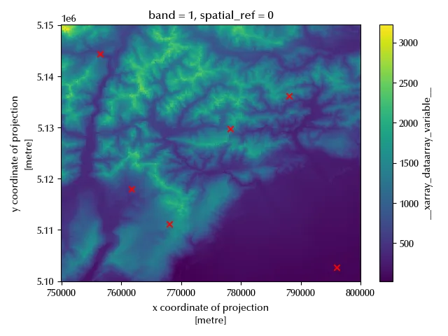
As we can see, we get a great spatial coverage with a small number of points. Since it can only be applied to rectangular regions, it cannot always be applied.
As previously mentioned, only spatial coverage random sampling both ensures a good spatial coverage and randomness.
Let us now take a look at the equidistant sampling method
dist = 0.05e6
pts, gdf_ed = draw_equidistant_points(geom, 5, [dist, dist/2, dist/4, dist/8], rng=rng)

fig, ax = plt.subplots()
geom.plot(ax=ax, color='lightgray')
gdf_ed.plot(column='scale',ax=ax, legend=True)
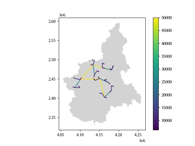
We can see 5 main points such that the distance between each point and the subsequent is constant and equal to 50 km. From each of the points we attached another point with distance equal to 25 km. From each of the above 10 points $x_0^i$, we sampled another point $x_1^i$, and their distance is equal to 12.5 km. We then sampled 20 points and their distance from the first 20 points is equal to 6.25 km, and we finally sampled 40 additional points with a distance equal to 3.125 km from the initial 40 points. In this way we are confident that our data will be appropriate to analyze the distance dependence on a scale going from roughly 3 km up to 25 km.
Conclusions
Also in this case we have seen that a sampling strategy might be more or less appropriate depending on your needs. Pure random sampling rarely finds application to spatial sampling, and it might be that grid sampling is sufficient for your task or that you need a more advanced sampling method, such as spatial coverage sampling or equidistant sampling.
%load_ext watermark
%watermark -n -u -v -iv -w
Python implementation: CPython
Python version : 3.12.8
IPython version : 8.31.0
numpy : 2.1.3
scipy : 1.15.2
rasterio : 1.4.3
matplotlib : 3.10.1
pandas : 2.2.3
geopandas : 1.0.1
sampling_tille: 0.1.5
seaborn : 0.13.2
Watermark: 2.5.0