

Spatial sampling
Data validation is a fundamental step for most applications, and this can be a very demanding step. Here we will discuss the most important spatial techniques for vector spatial data.
Sampling strategies
The simplest sampling method is, of course, simple random sampling, but this method has one major drawback when applied to spatial data: it does not ensure spatial coverage, and in GIS this is often more important than random data.
As we already discussed in our previous post a better approach is to use pivotal sampling, since this method ensure a better spatial coverage with respect to SRS.
In some cases, we can however do better, and in particular when you already know some quantity which correlates with the variable you are interested in. In these cases you can use the spread and balanced sampling techniques, which both enforces coverage and an unbiased estimate of the variable of interest.
Another popular strategy is to use generalized random tessellation sampling, which consists in the following procedure:
- We first assign to each point a selection probability, normalized in such a way that the sum of all the probabilities is equal to the sample size, and we drop all the points with zero probability
- We construct a rectangular grid around the study area
- we divide the grid into 4 equal cells, and we randomly assign a label 0,1,2 or 3 to each cell
- if any cell contains more than one point, we divide each cell into 4 sub-cells, we randomly select a number 0,1,2,3 for each subcell, and we append it to the label, and we repeat until all the cells contains at most one point
- We revert each label (0121 is transformed in 1210), and we sort all the non-empty cell according to it
- We compute the cumulative probability $\pi_i$ of each cell
- We generate a random number $u_0$ with uniform probability between 0 and 1 and we set \(u_1 = u_{0}+1,\dots,u_{n-1} = u_0 + n-1\)
- For each $k$, we select $i_k$ by choosing \(\min_{\pi_i} \pi_i \geq u_k\)
Let us compare these methods.
Sampling NY boros
We will now compare the above sampling methods by using a dataset provided by the center for spatial data science of the university of Chicago.
import pandas as pd
import numpy as np
import geopandas as gpd
import seaborn as sns
from matplotlib import pyplot as plt
from scipy.spatial import distance
from sampling_tille import sample_df, gdf_spread_balanced_sample, gdf_pivotal_sampling, gdf_edges_sample, sample_generalized_random_tessellation, load_data
import warnings

warnings.simplefilter("ignore")

gdf_ny = load_data('NewYork')
gdf = gdf_ny.to_crs('EPSG:5069')

fig, ax = plt.subplots()
gdf.plot(ax=ax)
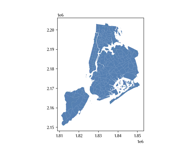
We will now construct a geodataframe using the centroids of the above dataset, and we will sample 15 points from it.
gdf1 = gdf.copy()
gdf1 = gdf1.set_geometry(gdf.centroid)

dt = 20250723

rng = np.random.default_rng(dt)

n = 15

m0 = sample_df(gdf1, n=n, rng=rng)

cols = ['poptot', 'popunemplo']

m1 =  gdf_pivotal_sampling(gdf1, rng=rng, n=n).astype(bool)

m2 = gdf_spread_balanced_sample(gdf1, n, balance=cols, rng=rng)

m3 = sample_generalized_random_tessellation(gdf1, gdf_bounds=gdf, n=n, rng=rng)

fig, ax = plt.subplots(ncols=4, figsize=(18, 12))

gdf.plot(ax=ax[0])
gdf1[m0].plot(ax=ax[0], color='k', marker='x')

gdf.plot(ax=ax[1])
gdf1[m1].plot(ax=ax[1], color='k', marker='x')

gdf.plot(ax=ax[2])
gdf1[m2].plot(ax=ax[2], color='k', marker='x')

gdf.plot(ax=ax[3])
gdf1[m3].plot(ax=ax[3], color='k', marker='x')
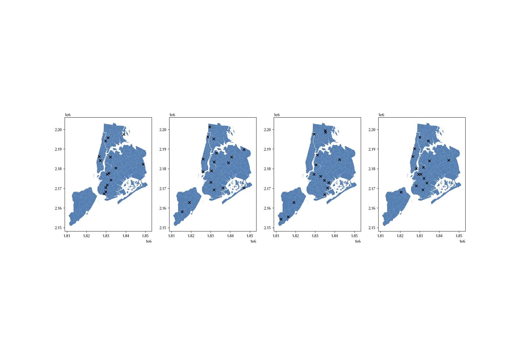
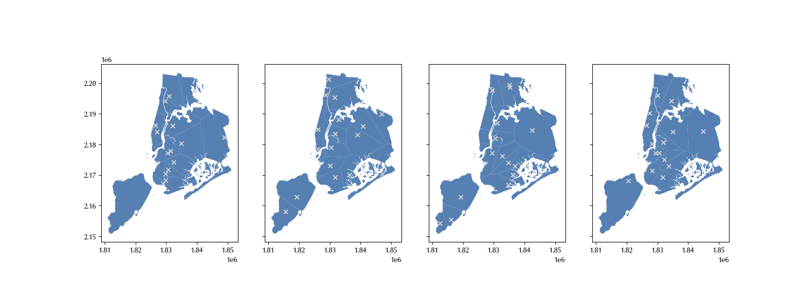
There are no points from Staten Island in the SRS sample, while the two remaining methods show a better coverage. We can better visualize this by looking at the Voronoi diagrams associated to our samples.
bds = gdf.union_all()
poly0 = gdf1[m0].voronoi_polygons().intersection(bds)
poly1 = gdf1[m1].voronoi_polygons().intersection(bds)
poly2 = gdf1[m2].voronoi_polygons().intersection(bds)
poly3 = gdf1[m3].voronoi_polygons().intersection(bds)

fig, ax = plt.subplots(ncols=4, figsize=(16, 6), sharey=True)
poly0.plot(ax=ax[0])
gdf1[m0].plot(ax=ax[0], marker='x', color='lightgray')
poly1.plot(ax=ax[1])
gdf1[m1].plot(ax=ax[1], marker='x', color='lightgray')
poly2.plot(ax=ax[2])
gdf1[m2].plot(ax=ax[2], marker='x', color='lightgray')
poly3.plot(ax=ax[3])
gdf1[m3].plot(ax=ax[3], marker='x', color='lightgray')
Let us now compare the expected value of the two selected columns:
gdf[cols].mean()
popunemplo 2190.082051
dtype: float64
gdf[m0][cols].mean()
popunemplo 2675.933333
dtype: float64
gdf[m1][cols].mean()
popunemplo 39145.588235
dtype: float64
gdf[m2][cols].mean()
popunemplo 39145.588235
dtype: float64
gdf[m3][cols].mean()
popunemplo 2301.800000
dtype: float64
The results in this case are quite clear, and only the last method provides an accurate estimate of the two quantities.
In order to perform a more reliable comparison, we will repeat few times the sampling, and visualize the results.
def get_simple_sample(gdf, n_pts, n_rep, cols):
    bds = gdf.union_all()
    gdf1 = gdf.copy()
    gdf1 = gdf1.set_geometry(gdf.centroid)
    out = []
    for _ in range(n_rep):
        m = sample_df(gdf1, n=n_pts)
        gdf_s = gdf1[m]
        true_means = gdf[cols].mean()
        sample_means = gdf_s[cols].mean()
        err = np.abs(sample_means-true_means).to_dict()
        poly = gdf_s.voronoi_polygons().intersection(bds)
        sd = np.std(poly.area/1e6)
        err.update({'area_sd': sd})
        out.append(err)
    return pd.DataFrame.from_records(out)

def get_pivotal_sample(gdf, n_pts, n_rep, cols):
    bds = gdf.union_all()
    gdf1 = gdf.copy()
    gdf1 = gdf1.set_geometry(gdf.centroid)
    out = []
    for _ in range(n_rep):
        # m = sample_df(gdf1, n=n_pts)
        m = gdf_pivotal_sampling(gdf1, n=n_pts).astype(bool)
        gdf_s = gdf1[m]
        true_means = gdf[cols].mean()
        sample_means = gdf_s[cols].mean()
        err = np.abs(sample_means-true_means).to_dict()
        poly = gdf_s.voronoi_polygons().intersection(bds)
        sd = np.std(poly.area/1e6)
        err.update({'area_sd': sd})
        out.append(err)
    return pd.DataFrame.from_records(out)

def get_spread_balanced_sample(gdf, n_pts, n_rep, cols):
    bds = gdf.union_all()
    gdf1 = gdf.copy()
    gdf1 = gdf1.set_geometry(gdf.centroid)
    out = []
    for _ in range(n_rep):
        # m = sample_df(gdf1, n=n_pts)
        m = gdf_spread_balanced_sample(gdf1, n=n_pts, balance=cols).astype(bool)
        gdf_s = gdf1[m]
        true_means = gdf[cols].mean()
        sample_means = gdf_s[cols].mean()
        err = np.abs(sample_means-true_means).to_dict()
        poly = gdf_s.voronoi_polygons().intersection(bds)
        sd = np.std(poly.area/1e6)
        err.update({'area_sd': sd})
        out.append(err)
    return pd.DataFrame.from_records(out)

def get_grts(gdf, n_pts, n_rep, cols):
    bds = gdf.union_all()
    gdf1 = gdf.copy()
    gdf_bds = gdf.copy()
    gdf1 = gdf1.set_geometry(gdf.centroid)
    out = []
    for _ in range(n_rep):
        # m = sample_df(gdf1, n=n_pts)
        m = sample_generalized_random_tessellation(gdf1, gdf_bds, n=n_pts).astype(bool)
        gdf_s = gdf1[m]
        true_means = gdf[cols].mean()
        sample_means = gdf_s[cols].mean()
        err = np.abs(sample_means-true_means).to_dict()
        poly = gdf_s.voronoi_polygons().intersection(bds)
        sd = np.std(poly.area/1e6)
        err.update({'area_sd': sd})
        out.append(err)
    return pd.DataFrame.from_records(out)

n_pts = 20
n_rep = 100

df_ss = get_simple_sample(gdf_ny, n_pts, n_rep, cols)

df_ps = get_pivotal_sample(gdf_ny, n_pts, n_rep, cols)

df_sb = get_spread_balanced_sample(gdf_ny, n_pts, n_rep, cols)

df_grts = get_grts(gdf_ny, n_pts, n_rep, cols)

def plot_comp(col):
    fig, ax = plt.subplots(ncols=4, sharey=True, figsize=(12, 4))
    sns.barplot(df_ss, y=col, x=df_ss.index, color='C0', ax=ax[0])
    sns.barplot(df_ps, y=col, x=df_ss.index, color='C0', ax=ax[1])
    sns.barplot(df_sb, y=col, x=df_ss.index, color='C0', ax=ax[2])
    sns.barplot(df_grts, y=col, x=df_ss.index, color='C0', ax=ax[3])
    ax[0].set_xticks([])
    ax[1].set_xticks([])
    ax[2].set_xticks([])
    ax[3].set_xticks([])
    ax[0].set_xlabel('Sample')
    ax[1].set_xlabel('Sample')
    ax[2].set_xlabel('Sample')
    ax[3].set_xlabel('Sample')
    ax[0].set_title('SRS')
    ax[1].set_title('Pivotal')
    ax[2].set_title('Spread balanced')
    ax[3].set_title('GRTS')
    ax[0].set_xticks([])
    fig.tight_layout()
    return fig

figs = [plot_comp(col) for col in df_ss.columns]
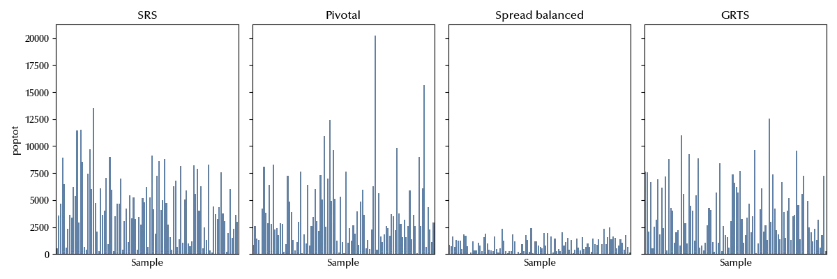
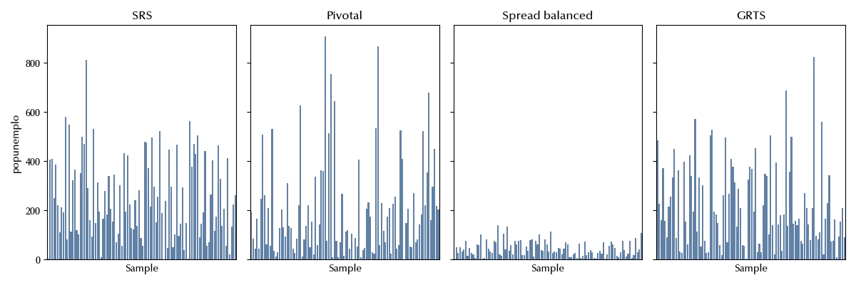
From the above figures, it’s clear that the spread balanced sampling method ensures a much more accurate estimate of the selected columns. Let us now compare the standard deviation of the Voronoi polygons.
df_ss['method']='SRS'
df_ps['method']='Pivot'
df_sb['method']='Spread Balanced'
df_grts['method']='GRTS'

df_plot = pd.concat([df_ss, df_ps, df_sb, df_grts])

bins = np.arange(0, 50, 1)
fig, ax = plt.subplots()
sns.kdeplot(df_plot, x='area_sd' , hue='method', ax=ax)
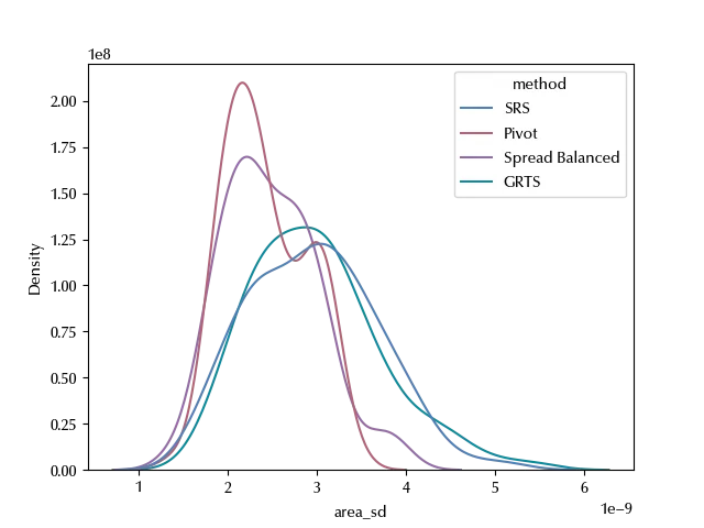
In the SRS case and in the GRTS one, the area dispersion is broader, while for the other sampling strategies it looks like the Voronoi of each sample have a closer area among themselves. The main difference between the GRTS sampling and the pivot/spread balanced sampling is that the GRTS method ensures that the spatial distribution represents the population spatial distribution, while the remaining methods ensures coverage. Those concepts are different if the point distribution is not uniform on space, and GRTS will ensure that denser areas contain more points. On the other hand, pivot/spread balance sampling strategies will ensure that points from both denser and looser areas are included in the sample.
Road sampling
We have used the above method to sample points, but we can easily adapt the above method to sample points from networks such as roads.
A uniform sample from a network road can be performed as follows
- we first sample a segment with probability proportional to its length
- we then sample a random point from the segment.
The above method can be easily adapted to perform a pivot sampling.
gdf_street = load_data('Palmanova')

npts = 15

pts0 = gdf_edges_sample(gdf_street, n=npts, kind='simple', rng=rng)
pts1 = gdf_edges_sample(gdf_street, n=npts, kind='pivotal_distance', rng=rng)

fig, ax = plt.subplots(ncols=2, figsize=(14, 4), sharey=True)
gdf_street.plot(ax=ax[0], alpha=0.4, color='lightgrey')
pts0.plot(ax=ax[0], color='C1', marker='x')
gdf_street.plot(ax=ax[1], alpha=0.4, color='lightgrey')
pts1.plot(ax=ax[1], color='C1', marker='x')
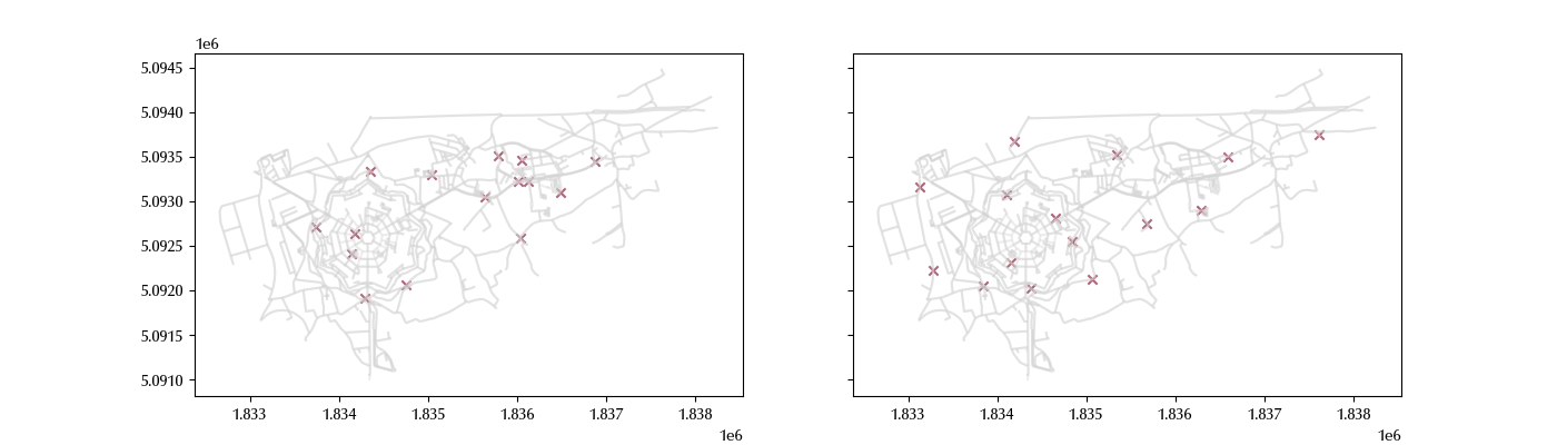
Notice that, for the moment, the above method uses the distance between the centroids as matrix distance, which is not the best distance we could use, since the minimum of the distance between the points of the edges would be more appropriate.
Conclusions
SRS is a valid sampling method, but you should always keep in mind that modern sampling techniques allow you to ensure a good spatial properties and, if needed, unbiased estimates of the desired quantities.
%load_ext watermark

%watermark -n -u -v -iv -w
Python implementation: CPython
Python version : 3.12.11
IPython version : 9.1.0
numpy : 2.3.1
matplotlib : 3.10.0
seaborn : 0.13.2
scipy : 1.15.2
pandas : 2.3.1
geopandas : 1.1.1
sampling_tille: 2.0.0
Watermark: 2.5.0