Random sampling

In the last post we briefly introduced the concept of random sampling. In this post we will discuss this topic with a little bit more of details, and see the advantages of probability sampling over non-probability sampling, as well as few design principles to design a proper sampling.

We will only discuss sampling without repetitions, since sampling with repetition gives worse performance and, in most situations, does not give any particular advantage.

Finite population sampling

Let us give a more precise definition of what a sampling strategy is. We restrict ourselves to finite population samples and to sampling without replacements, where the population is any finite set $$ P = \left\{ a_i \right\}_{i=1}^N $$ We define the sampling universe $$ U = \bigcup_i A_i $$ where $$ A_i \subset P\,. $$ Since each unit can or cannot be included in the sample, the size of $U$ is $2^N$. A sampling strategy is a map $$ p : U \longrightarrow [0, 1] $$ such that $$ \sum_i p(A_i) = 1\,. $$ In other words, a sampling strategy attaches a probability to each subset of the population.

Sampling principles

In a recent preprint Tillé proposed a set of principles to design a sampling strategy:

randomization
over-representation
restriction

We will now discuss these principles, and we will then see how they can be applied to different situations.

Randomization

Randomization is needed in order to gain the maximum amount of possible information. We recall that the information can be quantified via the entropy, and the larger the randomness, the higher the entropy. A greater randomness will therefore translate in a higher entropy. A higher information gain implies more robust conclusions, so we should choose the design with the highest amount of randomness among them compatible with the remaining principles, as well as with any other practical constrain.

This also implies that any unit should have non-zero probability of being included, but it does not necessarily mean that each unit should have the same probability of being selected.

Over-representation

A lot of people think that a good sample should look like the population, so any unit should have the same probability of being selected. This is however wrong, since we can and should also rely on any other source of available information when we draw our conclusion.

Including in our sample units which are already known to us is a complete waste of resources, while we should give a higher chance (or even the certainty) of being included in our sample to units which are highly uncertain. This is commonly done in company surveys, where larger companies give a larger contribute to the total variance, and are therefore always included in many surveys.

For the above reason, Tillé considers the concept of representativeness of a sample as a misleading concept, and I personally cannot disagree with him.

Restriction

When we draw a sample, we are always imposing some restriction. As an example, we often look for samples with a given number of items. Moreover, if we know that a particular quantity correlates with our target variable, we should constrain it in order to have a more precise estimate. Stratification can be considered as a constraint too, since we impose the number of units in the sample for each stratum. Restrictions are therefore needed in order to avoid bad samples, allowing us to focus on those samples which have a higher probability of giving us a good estimate of the target variable.

Sampling methods

We will now discuss the classical sampling designs, as well as few modern designs.

Simple random sampling

Simple random sampling without replacement is the simplest sampling strategy, and it is generally applied when there are no requirements regarding restriction or over-representation.

This designs assigns to each unit the same probability, and randomly selects $n$ units out of $N$ elements.

import pandas as pd
import geopandas as gpd
import numpy as np
from sampling.df_sample import sample
from sampling.load_data import load_data

n = 25

rng = np.random.default_rng(42)

df = load_data('Belgium')

m1 = sample(df, n=n, rng=rng)

df[m1].head()

	Commune	INS	Province	Arrondiss	Men04	Women04	Tot04	Men03	Women03	Tot03	Diffmen	Diffwom	DiffTOT	TaxableIncome	Totaltaxation	averageincome	medianincome
34	Heist-op-den-Berg	12014	1	12	18790	19144	37934	18725	18979	37704	65	165	230	435257229	116441471	25287	20399
47	Dessel	13006	1	13	4396	4329	8725	4363	4287	8650	33	42	75	97561973	24235869	24336	20212
77	Ganshoren	21008	2	21	9261	11372	20633	9129	11305	20434	132	67	199	240976682	67280446	24304	18891
140	Kortenberg	24055	2	24	8855	9118	17973	8741	9041	17782	114	77	191	259079443	82351738	32704	23994
208	Courtrai	34022	3	34	36076	37798	73874	36311	37988	74299	-235	-190	-425	918625170	253525983	25402	19079

Cluster sampling

Cluster sampling relies on randomization, and it is a less efficient sampling strategy with respect to simple random sampling. Cluster sampling selects all the units from one or more clusters, and is generally used when sampling from different clusters requires more effort than sampling from the same cluster.

This often happens when, in order to perform the sampling, you must move from one place to another in order to change cluster.

In our case, we will use “Arrondiss” as a clustering column.

np.mean(df.groupby(['Arrondiss'])['Commune'].count())

np.float64(13.69767441860465)

There are, on average, 14 municipalities in each arrondissment, so if we select 2 municipalities we should have a number of sampled units which is not too far away from our target sample size. This is one of the main drawbacks of cluster sampling, since it does not allow to select the sample size. The other main drawback is that it might happen that units within the same cluster are more similar than units coming from different clusters, so a sample obtained by cluster sampling with a given size might contain less information than a sample with the same size obtained by using simple random sampling.

m2 = sample(df, n=n // 10, rng=rng, kind='cluster', columns=['Arrondiss'])
# We prefer a little bit more of units than a little bit less

len(df[m2])

df[m2]['Arrondiss'].drop_duplicates()

30 12
204 34
Name: Arrondiss, dtype: int64

We assigned to each cluster the same probability, but in some situation it might be a good idea to assign different probabilities to different cluster. As an example, you might desire to assign a probability proportional to the number of units in the cluster, and this can be done with the method=size option.

Stratified random sampling

Stratification is a common technique to group units which have similar characteristics.

Stratified random sampling is an improvement over simple random sampling, and it’s used when you want to make sure that your sample includes units from all of your strata.

This is the first application of the over-representation principle, since we demand that our sample contains units from all of our strata. Since our design ensures that all groups are included in our samples, if the stratification is performed on variables that contribute to the variance of our target variable, this design ensures a higher amount of information with respect to the simple random sampling.

m3 = sample(df, n=20, rng=rng, kind='stratified', columns=['Province'])
df[m3].groupby('Province')['Commune'].count()

Province
1 2
2 4
3 2
4 2
5 2
6 3
7 1
8 1
9 1
Name: Commune, dtype: int64

As you can see, our sample contains units from all the provinces. Let us compare the distribution of the provinces in this sample with the same distribution for the simple random sample.

dfa = df[m1].groupby('Province')['Commune'].count()/len(df[m1])
dfb = df.groupby('Province')['Commune'].count()/len(df)
dfc = df[m3].groupby('Province')['Commune'].count()/len(df[m3])

dfa = dfa.reset_index()
dfb = dfb.reset_index()
dfc = dfc.reset_index()

dfa['Sample'] = 'simple'
dfb['Sample'] = 'total'
dfc['Sample'] = 'stratified'

df_frac = pd.concat([dfa, dfb, dfc])

df_frac.rename(columns={'Commune': 'Fraction'}, inplace=True)

fig, ax = plt.subplots()
sns.barplot(df_frac, x='Province', y='Fraction', hue='Sample', ax=ax, legend=True)
ax.set_yticks([0, 0.1, 0.2])
ax.set_title('Percentage of municipalities per province')
legend = ax.legend()
legend.get_frame().set_alpha(0)
fig.tight_layout()

The comparison of the distribution of the number of provinces
between the total population, the simple random sample
and the stratified random sample.

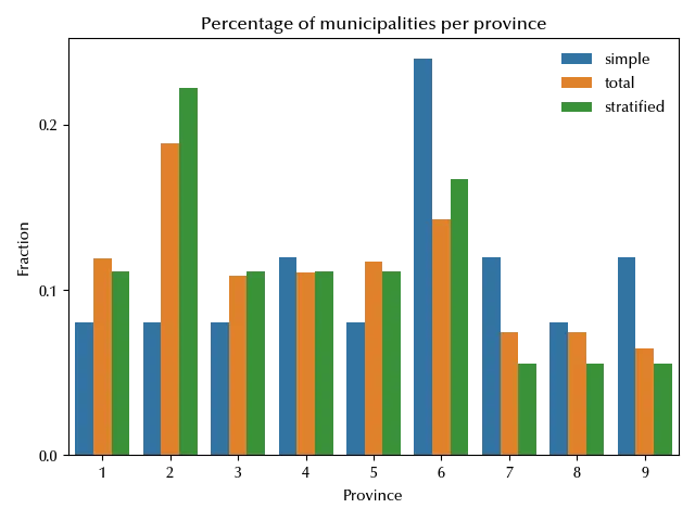
In the stratified sample, the provinces are distributed as they are in the original sample, while in simple random sampling there are provinces which are present in a higher percentage and provinces which are present in a lower percentage.

We could however choose and impose another distribution. A common situation is one when you want to estimate with the same precision a parameter for each stratum, and in this case fixing the same number of units for each stratum is a good choice. This can be done with the option method=equal_size.

Systematic sampling

In the stratified sampling design we saw how to ensure that each one of a set of different classes is represented into our sample, and the same concept can be immediately generalized by stratifying with respect to more than one categorical variable.

If however we want to ensure that the entire range of values of a continuous variable is present in our sample, we cannot straightforwardly apply the above strategy.

The possible choices in this case are two: we can either discretize the continuous variables, either by using equally spaced subsets or more advanced methods ¹, or we can use some form of systematic sampling. The basic form of systematic sampling is very easy, and it can be done in four steps:

We compute k=n//N and l=n%N
We sort our dataframe according to the column we want to stratify on
We sample a random number i between 0 and k-1
we take the units i, i+k, i+2k,…,i+(l-1)*k

Alternatively, we can use

col = 'medianincome'

df_sort = df.sort_values(by=col, ascending=True)

m4 = sample(df_sort, n=n, rng=rng, kind='systematic')

Before discussing the results of the systematic sampling strategy, let us introduce a more recent sampling design, namely the pivotal method.

Pivot sampling

Pivotal sampling has been first developed by Deville and Tillé in 1996 in this paper.

With this method, in each step, we then apply the following algorithm:

Select a random unit $i$ among those with $0 < \pi_i < 1$
Find its nearest neighbour $j$ among those with $0 < \pi_j < 1$
If $\pi_i + \pi_j > 1$ then:
1. generate $0 \leq \lambda \leq 1$ uniformly
2. if $\lambda < \pi_i/(\pi_i + \pi_j)$ set $\pi_i$ to 1 and $\pi_j$ to $(\pi_i + \pi_j -1)$, otherwise switch $i$ and $j$
If $\pi_i + \pi_j <= 1$ then:
1. generate $0 \leq \lambda \leq 1$ uniformly
2. if $\lambda < \pi_i/(\pi_i + \pi_j)$ set $\pi_j$ to 0 and $\pi_i$ to $(\pi_i + \pi_j)$, otherwise switch $i$ and $j$.

The effect is analogous to the one we would have obtained by using a systematic sampling sorting with respect to $x$. We can however generalize the above concept and use any distance matrix for $x$ either one dimensional or multidimensional, so this method can be also applied to spatial sampling.

The above method has been improved by verifying in step 2 that $i$ is the nearest neighbour of $j$. If it is, then step 3 is performed, otherwise one goes back to step 1.

One of the great advantages of the (local) pivot method over the systematic sampling is that systematic sampling implies the sorting with respect to one variable, while the pivot methods look for the nearest neighbour, which is a well define concept in more than one dimension too.

m5 = sample(df, n=n, kind='pivotal', columns=[col], rng=rng)

fig, ax = plt.subplots(ncols=4, figsize=(9, 4), sharey=True)
sns.violinplot(df, y=col, ax=ax[0])
sns.violinplot(df[m1], y=col, ax=ax[1])
sns.violinplot(df_sort[m4], y=col, ax=ax[2])
sns.violinplot(df[m5], y=col, ax=ax[3])
sns.swarmplot(df, y=col, ax=ax[0],  size=3)
sns.swarmplot(df[m1], y=col, ax=ax[1], size=3)
sns.swarmplot(df_sort[m4], y=col, ax=ax[2],  size=3)
sns.swarmplot(df[m5], y=col, ax=ax[3],  size=3)
ax[0].set_title('Population')
ax[1].set_title('SRS')
ax[2].set_title('Systematic')
ax[3].set_title('Pivot')
ax[0].set_ylim([10000, 27500])
ax[1].set_ylim([10000, 27500])
ax[2].set_ylim([10000, 27500])
ax[3].set_ylim([10000, 27500])
fig.tight_layout()

The violin plot and the swarm plot of the median income
for the simple random sample, the true population,
the systematic sampling and the pivot method

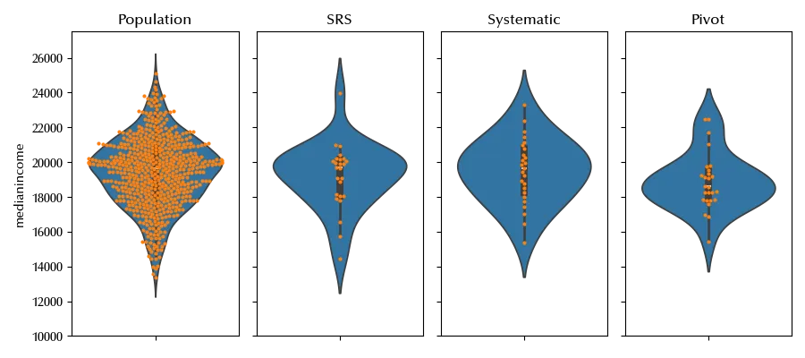
The last two methods enforce a balanced distribution of the target variable, while this balance is not guaranteed by using simple random sampling.

Balanced sampling

Balanced sampling is a powerful method, and it constrains the average value of one or more variables to a value close to average population one. This can be very useful to obtain an unbiased estimate of your target variable $y$ if you can balance with respect to a variable $x$ which is strongly correlated with $y$. Balanced sampling is ensured by using the cube method, which is a quite complicated sampling algorithm. The interested reader is invited to read Tillé’s textbook for more details on the cube sampling.

Since the fraction of a binary variable is the sample average, balancing on a discrete variable is equivalent to stratify over it.

Moreover, the sample size is enforced as the average of the identically 1 variable.

Let us take at an example where we balance on four columns

m6 = sample(df, n=n, rng=rng, kind='balanced', balance=['Men03', 'Women03', 'Men04', 'Women04'])


df_plot = pd.DataFrame({'sample': ['Population', 'SRS', 'Balanced'], 
                        'Men03 avg': [df['Men03'].mean(), df[m1]['Men03'].mean(), df[m6]['Men03'].mean()],
                        'Men04 avg': [df['Men04'].mean(), df[m1]['Men04'].mean(), df[m6]['Men04'].mean()],
                        'Women03 avg': [df['Women03'].mean(), df[m1]['Women03'].mean(), df[m6]['Women03'].mean()],
                        'Women04 avg': [df['Women04'].mean(), df[m1]['Women04'].mean(), df[m6]['Women04'].mean()],
                       })

fig, ax = plt.subplots()
sns.barplot(df_plot.melt(id_vars='sample', value_vars=['Men03 avg', 'Men04 avg', 'Women03 avg', 'Women04 avg'],
var_name='quantity', value_name='value'), x='quantity', y='value', hue='sample', ax=ax)
legend = ax.legend()
legend.get_frame().set_alpha(0)
legend.set_bbox_to_anchor([1, 1])

fig.tight_layout()

The comparison of the men and women average value in 2003 and 2004
for the total population, the simple random sample
and the balanced sample

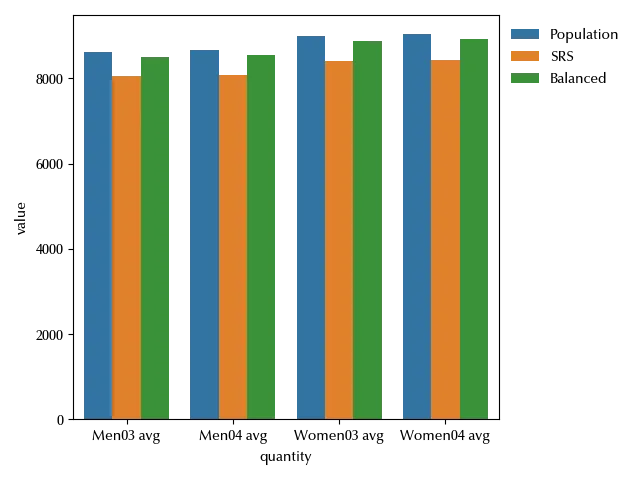
As we can see, the average values for the balanced sample are much closer to the population one than the ones obtained by using a simple random sampling design. The main issue of this method is that it is computationally intensive, and the computational effort grows very fast as the population size grows, so it can hardly be used when the population goes over few thousands units.

Conclusions

We discussed the sampling design principles proposed by Tillé, as well as some classical sampling method together with some modern sampling design. We saw how to use these methods in Python, and we compared the results of the different sampling design with respect to their underlying ideas.