
Stratification
As we saw in the last post, stratification can be very a very useful tool in survey design. There are however many practical issues in stratification, and here we will discuss some of them.
If you want to stratify with respect to a single categorical variable, you already know that the different strata are well separated, and you are confident that the number of strata is not too big, them you can simply move forward.
This is not always case, and here we will discuss how to stratify when the above conditions do not apply. While in R there are many packages to deal with this problem, first of all the stratification package, an analogous Python package was missing, so we included some of the routines in Python.
Binning your variable
If you want to stratify with respect to a single continuous variable, then binning is the first idea you might come out with.
When you bin, you simply divide the range of your variables into a given number of equally spaced segments. This is a very naive method, and it often works, but it is only appropriate if your variable has a finite range.
Let us see how to do this
import numpy as np
import pandas as pd
import seaborn as sns
from matplotlib import pyplot as plt
from sampling_tille.stratify import stratify_square_root, stratify_bins, stratify_geom, stratify_quantiles
from sampling_tille.load_data import load_data

df = load_data("Belgium")

sns.histplot(df["averageincome"], kde=True)
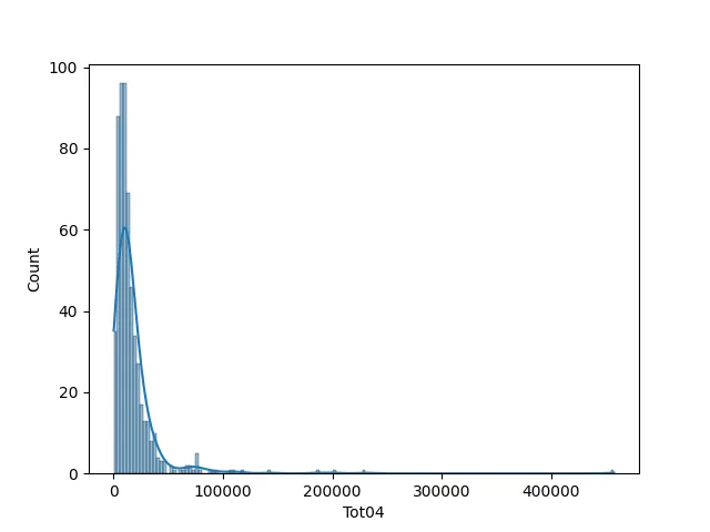
col = "Tot04"

strata_bins = stratify_bins(df[col], num_strata=5)
Using quantiles
A more sophisticated idea is to divide the population into segments with equal quantiles. In other words, you split the histogram of your variables into pieces with equal area. For a uniformly distributed variable, this method is equivalent to the one above. This method is more flexible than the one above, but it might cause issues with highly skewed quantities. In this case, it might be more appropriate to construct a stratum with fewer units, and always include them into the sample, since their contribution to the variance might be much larger than the one of the remaining strata. This method is often applied by economists, as in many surveys larger companies are included into the sample with probability 1.
This method can be easily implemented as follows
strata_quant = stratify_quantiles(df[col], num_strata=5)
The geometric progression
This very simple method has been used for a long time due to its simplicity, and it has been explicitly designed to handle skewed data. This method requires three inputs:
- the minimum value of the variable to stratify in the population $k_m$
- the maximum value of the variable to stratify in the population $k_M$
- the number of strata
By assuming that the strata boundaries are distributed according to a geometric succession, that the first bound is given by $k_m$ and the last bound by $k_M$, we get:
\[k_h = k_m \left(\frac{k_M}{k_m}\right)^{h/H}\]This method can be used by using
strata_geom = stratify_geom(df[col], num_strata=5)
Square root frequency stratification
The cumulative square root frequency stratification has been proposed in the fifties in order to provide an approximate way of obtaining strata with the same variance.
With this method we first divide the sorted dataset into a large number of classes, and we then compute the cumulative sum of the square root of the frequencies. We can then impose that the strata have equal intervals of the cumulative sum of the square root of the frequency.
strata_sr = stratify_square_root(df[col], num_strata=5)
Comparing the stratification methods
Let us now take a look at how the above stratification strategies performed
fig, ax = plt.subplots(nrows=2, ncols=2, sharex=True, sharey=True,
                       figsize=(11,11), squeeze=True)
sns.swarmplot(x=df[col], hue=strata_bins, ax=ax[0][0], log_scale=True)
sns.swarmplot(x=df[col], hue=strata_quant, ax=ax[0][1], log_scale=True)
sns.swarmplot(x=df[col], hue=strata_geom, ax=ax[1][0], log_scale=True)
sns.swarmplot(x=df[col], hue=strata_sr, ax=ax[1][1], log_scale=True)
ax[0][0].set_title("Bin stratification")
ax[0][1].set_title("Quantiles stratification")
ax[1][0].set_title("Geometric stratification")
ax[1][1].set_title("Square root stratification")
fig.tight_layout()
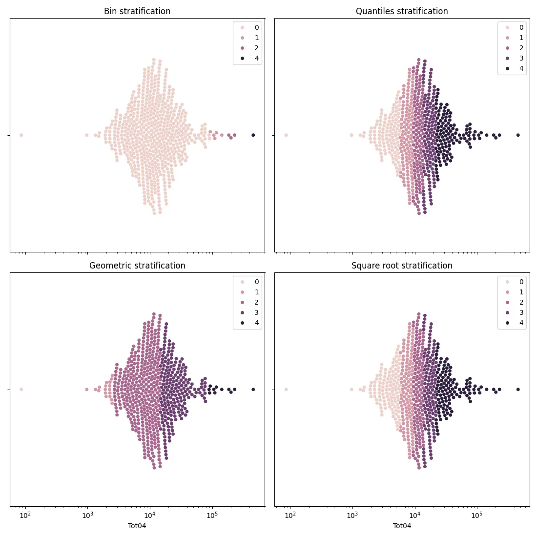
The stratum number three is empty for the binning strategy, and the first bin only has one element for the geometric method. While these methods are easy to implement, they can cause problems, so we don’t generally recommend them. On the other hand, the square root stratification and the quantile stratification give very similar results, and the distribution of the number of elements per stratum is balanced.
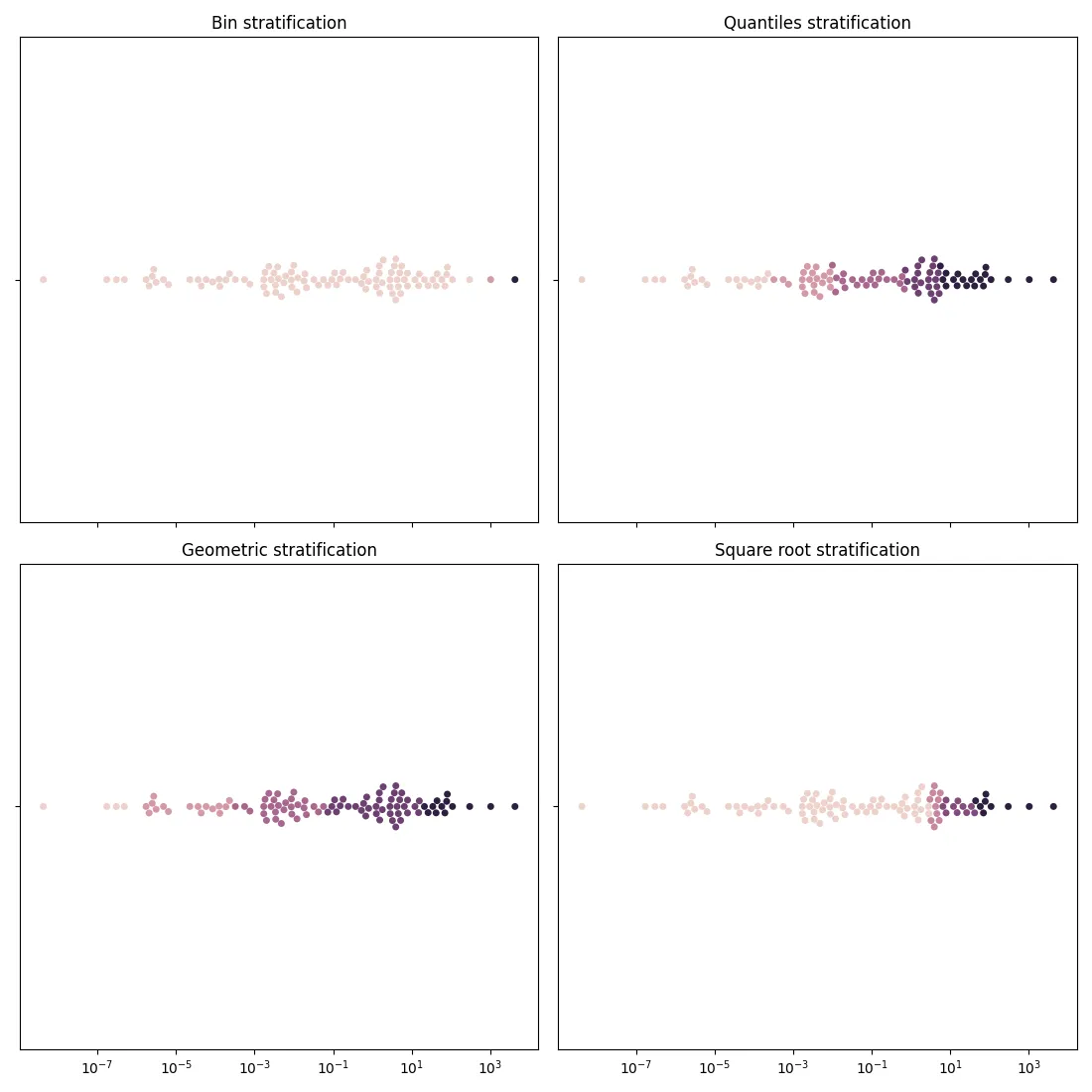
One might ask why we should implement the more involved square root method when the quantile method gives almost identical results. There are situations where the quantile method fails, in the sense that the higher strata span a too wide range, and this happens when the underlying distribution has heavy tails.
rng = np.random.default_rng(42)
xn = rng.weibull(0.25, size=100)

s0 =stratify_bins(xn, num_strata=5)
s1=stratify_quantiles(xn, num_strata=5)
s2=stratify_geom(xn, num_strata=5)
s3=stratify_square_root(xn, num_strata=5)

fig, ax = plt.subplots(nrows=2, ncols=2, sharex=True, sharey=True,  squeeze=True, figsize=(11, 11))
sns.swarmplot(x=xn, hue=s0, ax=ax[0][0], log_scale=True, legend=False)
sns.swarmplot(x=xn, hue=s1, ax=ax[0][1], log_scale=True, legend=False)
sns.swarmplot(x=xn, hue=s2, ax=ax[1][0], log_scale=True, legend=False)
sns.swarmplot(x=xn, hue=s3, ax=ax[1][1], log_scale=True, legend=False)
ax[0][0].set_title("Bin stratification")
ax[0][1].set_title("Quantiles stratification")
ax[1][0].set_title("Geometric stratification")
ax[1][1].set_title("Square root stratification")
fig.tight_layout()
Conclusions
We discussed pros and cons of some of the most common stratification method for univariate stratification. We have seen that the square root method generally gives better results than anyone of the methods discussed here. We finally saw how to implement these methods in python.