Design of experiments

Finding the best machine-learning algorithm is a common task in the data scientist job, and there are tons of tools which are available for this task. However, in most cases, they are unnecessary, and you can replace an azure experiment or a scikit-learn grid search with simpler tools which are less time-consuming and more transparent. Let us see how we can use the DOE principles in this kind of tasks with an example. We will also compare different strategies to tackle the problem, and we will discuss the main risks we run when we stick to too simplistic methods. While the following example is taken from the daily routine of a DS who is often involved into ML tasks, the same conclusions can be applied to any kind of decision.

A hypothetical example

Imagine you have a given dataset, and you must decide whether to replace a ML algorithm which performs a binary classification task. After discussing with the business, you decide that the precision is the most appropriate KPI for this problem. The deployed algorithm is a support vector machine classifier which uses an RBF kernel, but you guess that a polynomial kernel would do a better job.

You therefore decide to perform an experiment. Since the dataset is quite large, you don’t want to use too many trials, but you just want to perform enough trials to be sure that 9 times out of 10 you will be able to find the best algorithm. Your boss tells you that the RBF kernel have a precision of 0.9, and you reply that the linear kernel would lead to an improvement of 0.05. You therefore decide to perform a power analysis on your guesses, by using a value for alpha of 0.05, because that’s the value written in Fisher’s book, so ipse dixit! Your guess for the value of the standard deviations is 0.02 for both of them, and you assume that they are both normally distributed. Of course, you are aware that this does not take into account for the threshold effect (the precision cannot exceed 1), but in your opinion you are distant enough from this value and this issue should not affect your conclusions. You split multiple times the given dataset into a train set and a test set, and the one with the highest precision will be the winner. The null hypothesis is that the linear kernel does not perform better that the RBF kernel.

In the DOE jargon we have that a train-test split is considered an experimental unit, the kernel is the experimental factor and its values, RBF and polynomial, are the factor levels. The experimental units are randomly sampled from our target population, which is the set of all the possible train-test splits of our dataset. We should also consider that we are running the experiment with a specific experimental setting, namely my personal computer, which has a specific hardware (intel i7) and it’s running with a specific operating system (arch linux) with a specific Python version (3.13), with a given set of background tasks…

from ucimlrepo import fetch_ucirepo 
from sklearn.model_selection import train_test_split
from sklearn.svm import SVC
from sklearn.metrics import f1_score, precision_score
import numpy as np
import seaborn as sns
from matplotlib import pyplot as plt
from scipy.stats import ttest_ind, ttest_rel
import warnings
import pymc as pm
import arviz as az
import bambi as bmb
import pandas as pd

warnings.filterwarnings('ignore')

rng = np.random.default_rng(42)

kwargs = {'nuts_sampler': 'numpyro', 'random_seed': rng,
          'draws': 4000, 'tune': 4000, 'chains': 4, 'target_accept': 0.95}

def fpw(n):
    y1 = rng.normal(loc=0.9, scale=0.02, size=n)
    tau = rng.normal(loc=0.05, scale=0.02, size=n)
    y2 = y1+tau
    return ttest_ind(y1, y2, alternative='less')

predicted_power = np.mean([fpw(5).pvalue<0.05 for _ in range(1000)])
predicted_power

0.958

Our guess for the parameters gives us a power of 0.96, so 5 is a large enough number of trials. We will use the phishing dataset from the UCI ML repo dataset to simulate the given dataset.

SIZE = 5

dataset = fetch_ucirepo(id=327)  

Xs = dataset.data.features 
ys = dataset.data.targets 

def feval(x):
    score = precision_score
    Xtrain, Xtest, ytrain, ytest = train_test_split(Xs, ys, random_state=x)
    cls1 = SVC(kernel='rbf')
    cls1.fit(Xtrain, ytrain)
    ypred1 = cls1.predict(Xtest)

    cls2 = SVC(kernel='poly')
    cls2.fit(Xtrain, ytrain)
    ypred2 = cls2.predict(Xtest)
    
    score1 = score(y_true=ytest, y_pred=ypred1)
    score2 = score(y_true=ytest, y_pred=ypred2)
    return score1, score2

np.random.seed(100)

yobs = np.array([feval(np.random.randint(10000)) for _ in range(SIZE)]).T

fig, ax = plt.subplots(nrows=2)
sns.histplot(yobs[0], ax=ax[0])
sns.histplot(yobs[1], ax=ax[1])

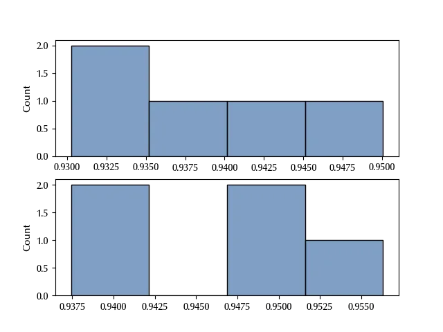
The performances of the two algorithms

ttest_ind(yobs[0], yobs[1], alternative='less')

TtestResult(statistic=-1.5339994511337103, pvalue=0.08178696565867705, df=8.0)

The bad news is that the above analysis did not show any difference between the performances of the two algorithms, so your guess appears wrong. The good news is that you were right, and you just failed to formulate the problem.

If we take a closer look at the procedure, we realize that we are comparing the performances of two different ML algorithms on the same dataset split. We could therefore compare the treatment effect (changing the classification algorithm) on each unit rather than on the entire sample. This might reduce the performance variability generated by the differences among the splits. If in fact in a train set there are too few examples of a certain type, we might expect that both the algorithms would have bad performances in classifying that kind of entry. Since that effect both shows in the RBF performance and in the polynomial one, when the comparison is performed unit by unit, that noise does not appear, but it does appear when we compare the average performances across all the experiment runs. A better way to isolate the treatment effect would be to run a one-sided paired t-test:

ttest_rel(yobs[0], yobs[1], alternative='less')

TtestResult(statistic=-7.111454171194376, pvalue=0.001033002027527698, df=4)

In this case the effect is clearly visible, with a p-value of $10^{-3}\,.$ This is why blocking is important, as a more meaningful comparison allows you to better isolate the effect despite the variability across units. But is it really a meaningful improvement? Let us take a look by using PyMC.

The model building perspective

Translating the different testing procedures into models is easy. In the first case we have

with pm.Model() as lm:
    mu1 = pm.Normal('mu', mu=0, sigma=10)
    theta = pm.Normal('theta', mu=0, sigma=10)
    sigma = pm.HalfNormal('sigma', 10)
    y1 = pm.Normal('y1', mu=mu1, sigma=sigma, observed=yobs[0])
    y2 = pm.Normal('y2', mu=mu1+theta, sigma=sigma, observed=yobs[1])

with lm:
    idata = pm.sample(**kwargs)

az.plot_trace(idata)
fig = plt.gcf()
fig.tight_layout()

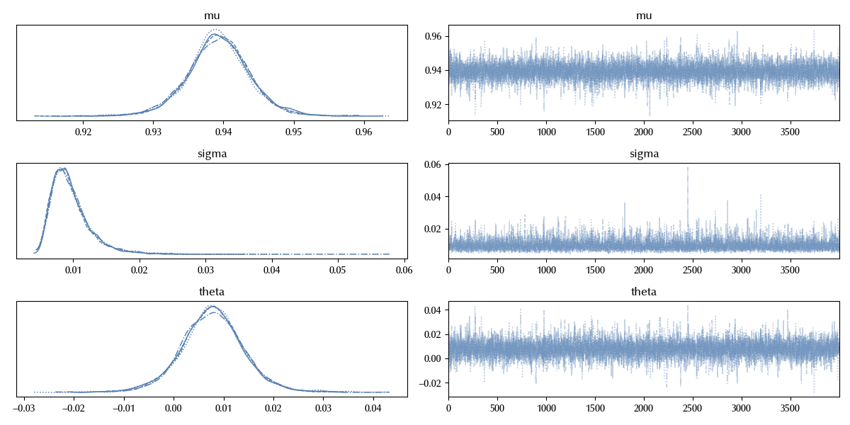
The distribution of $\theta$ clearly overlaps zero, we cannot therefore rule out the hypothesis that the performances of the polynomial kernel are not better than the ones of the RBF kernel.

The implementation of the above model in Bambi is straightforward. We must first of all encode the relevant data inside a pandas dataframe

df_data = pd.DataFrame({'ind': 2*list(range(len(yobs[0]))),
                        'trt': [0]*len(yobs[0])+[1]*len(yobs[0]),
                        'y': list(yobs[0])+list(yobs[1])})

df_data

	ind	trt	y
0	0	0	0.950063
1	1	0	0.94377
2	2	0	0.939319
3	3	0	0.933076
4	4	0	0.930247
5	0	1	0.956329
6	1	1	0.950128
7	2	1	0.951402
8	3	1	0.940039
9	4	1	0.93742

Once this is done, we must simply run

lm_bambi = bmb.Model('y ~ 1 + trt', data=df_data)

idata_lm = lm_bambi.fit(**kwargs)

az.plot_trace(idata_lm)
fig = plt.gcf()
fig.tight_layout()

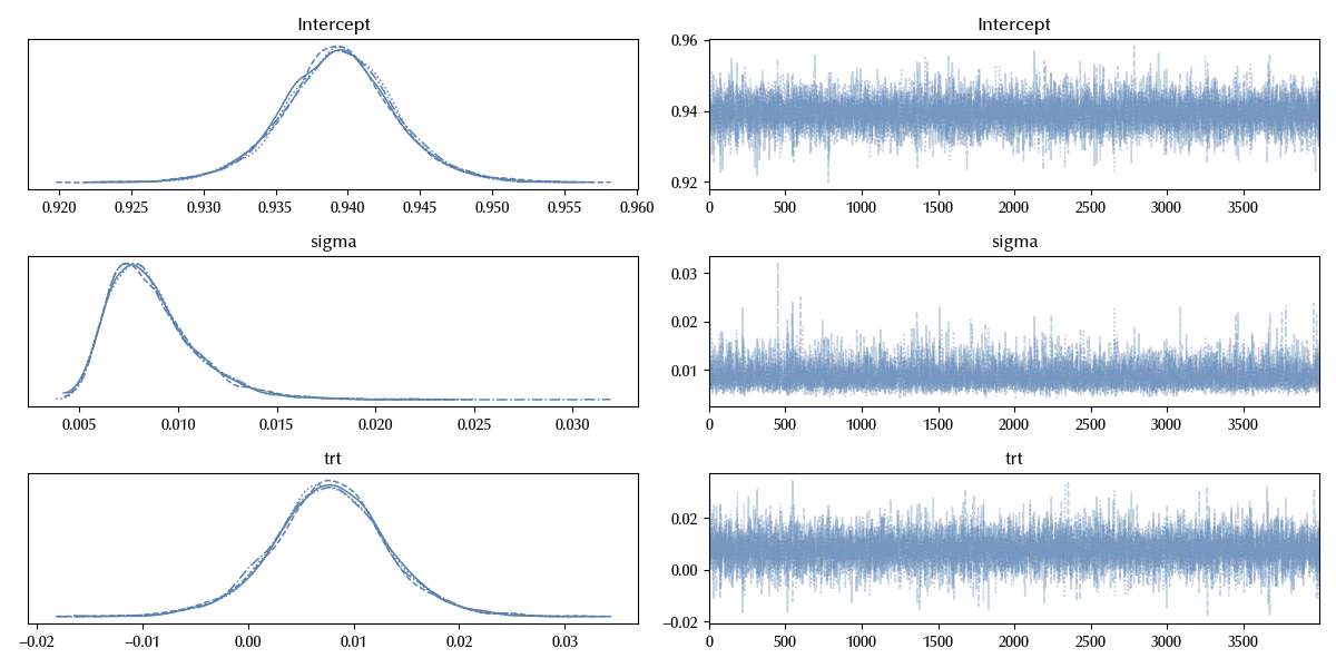
The trace of the same model implemented with Bambi

The results are clearly identical, as it should be.

Since the performances are evaluated by using the same train-test split, we could however simply model the performance difference of the two algorithms. A minor drawback of this approach is that it doesn’t tell us anything about the performances of the algorithms, as it only involves the performance difference. We can easily build a model which allows us to both encode the fact that the units are the same and to extract the performances of the one model, which will be our baseline, and we will do this with Bambi

lm_blocked = bmb.Model('y ~ ind + trt', data=df_data, categorical=['ind'])

idata_lm_blocked = lm_blocked.fit(**kwargs)

az.plot_trace(idata_lm_blocked)
fig = plt.gcf()
fig.tight_layout()

The trace of the new model

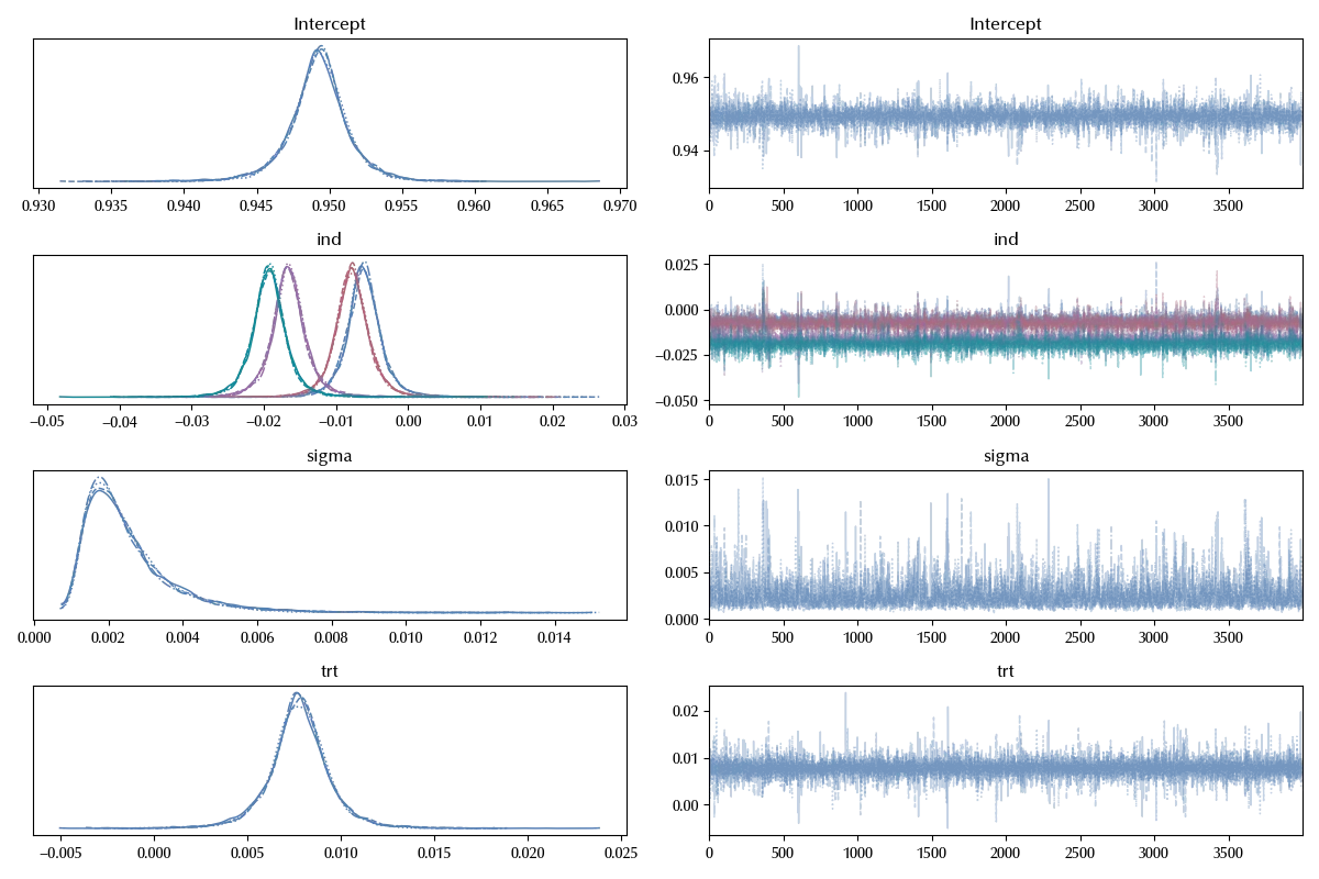
This models has a very large amount of information with respect to the previous ones:

The average score of the RBF algorithm (Intercept)
The average improvement of the polynomial kernel with respect to the RBF kernel (trt)
The variance due to the split variability (sigma)
The effect of each split on the RBF performance (which we assume being the same effect we observe on the polynomial) (ind)

A final improvement can be obtained by treating the train-test split effect as a random effect, and this also allows us to extract the variance due to the train-test split.

lm_blocked_h = bmb.Model('y ~1 + (1|ind) + trt', data=df_data, categorical=['ind'])

idata_lm_h = lm_blocked_h.fit(**kwargs)

az.plot_trace(idata_lm_h)
fig = plt.gcf()
fig.tight_layout()

The trace of the final model

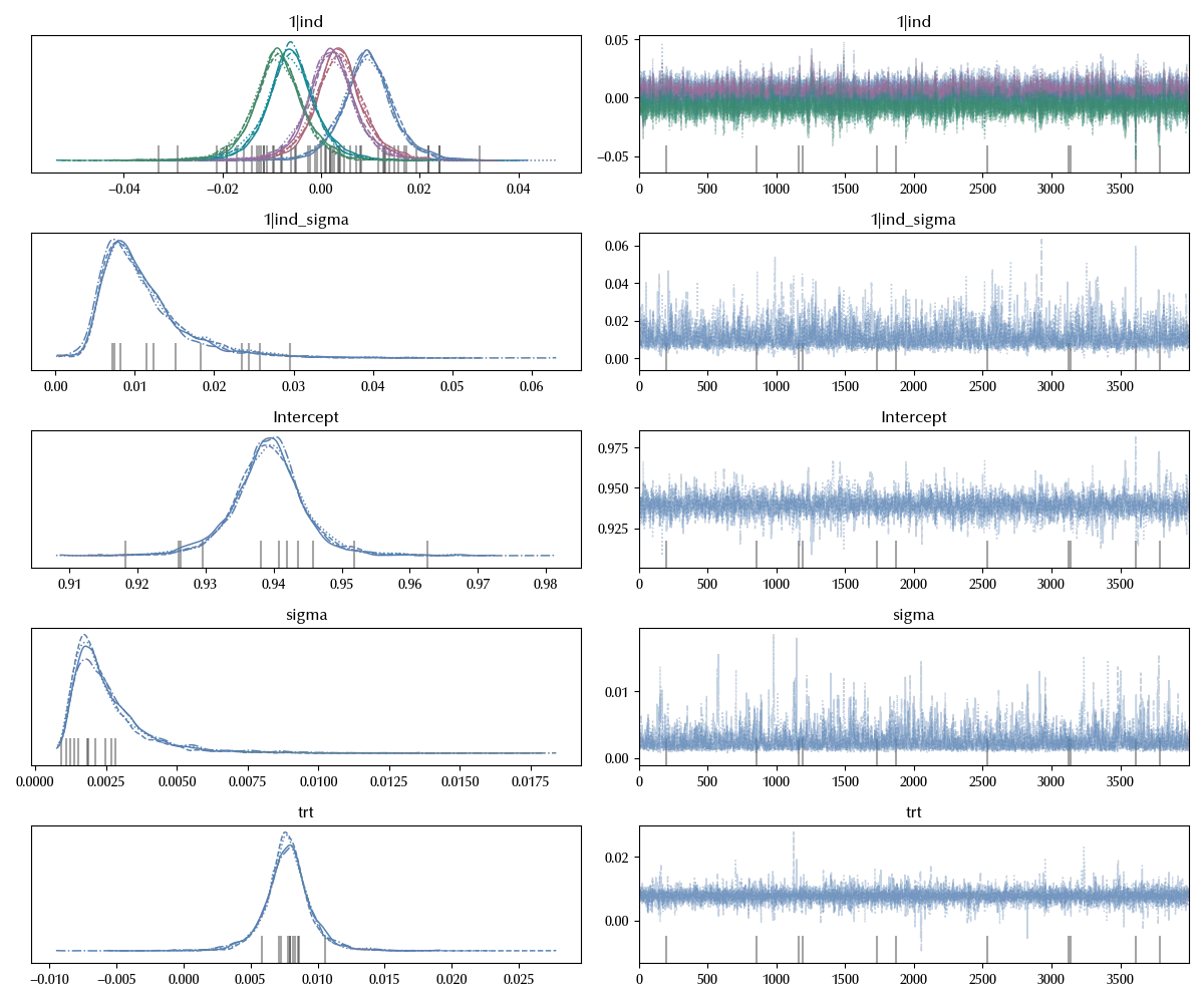
Being able to quantify all these parameters has the practical advantage that we can have a broader perspective on the problem we are trying to solve, and this can be really important when we analyze complex real world problems. In our case, we are now able to compare the estimated average treatment effect with the train-test split variance.

(idata_lm_h.posterior['trt']<idata_lm_h.posterior['1|ind_sigma']).mean().values

array(0.697125)

Since their magnitude is compatible, and since the treatment effect is also negligible with respect to the baseline, we must conclude that we have no particular advantage in terms of model performances in choosing one particular algorithm, and our choice should be based on a different criterion.

This is what statisticians mean when they say that an appropriate model is the one which encodes the desired amount of structure. A too simple model is risky as it could drive us in taking decisions on the basis of a part of the relevant information while hiding another relevant part. Using a statistical test can be even riskier when taking complex decision, unless we are not really sure that we are asking the exact question we want to investigate before the data collection (looking for the question once you have analyzed the data is not considered a good practice, as it leads to data dredging, p-value hacking and other dangerous practices).

In our case the first test, as well as the equivalent first model, would lead to wrongly accept the null hypothesis. In the second case, we would however perform an error of the third kind, since the improvement in the performances would hardly bring any value, while forcing us to spend time in the deployment of the new model.

We should always keep in mind that, when the statistical tests have been proposed, there were no computers available, and so it was fundamental to stick to simple tools in order to allow anyone to use statistics to make decisions. Fortunately, things have changed in the last century, and now anyone with the theoretical knowledge and with a sufficient amount of practice can easily design and implement an ad-hoc model for his/her own problem.

Conclusions

Asking the wrong question can lead you to take the wrong choice, therefore it is fundamental to only analyze the data once you are sure you understood the problem and the data.

Being able to quantify all the relevant aspects of a problem can be helpful in using data to take informed decisions, so it’s important not to oversimplify the problem. Encoding the correct amount of structure into our model is therefore crucial when we want to apply statistics to complex real-world problems.

A hypothetical example

The model building perspective

Conclusions

Suggested readings