

Radar interferometry with Pygmtsar
Before starting, I would like to warn the reader that this is an advanced topic, even for someone who worked if physics. I will try and make this topic as accessible as I can without over-simplifying.
Introduction to DINSAR
Differential SAR interferometry is a cutting-edge technique used by researchers to quantify the ground displacement. Up to now we only used the measured reflected amplitude, but SAR satellites such as Sentinel 1 are capable of measuring the phase too. If you had a course in optics, you might remember that the phase is determined by the length of the optical path. This means that, if we perform two subsequent phase measurements of the same region by keeping all the remaining conditions identical we can determine the ground displacement. Since SAR satellites can perform phase measurements with a very high precision, this method allows us to quantify ground displacements with a millimetric precision.
The one depicted above is the ideal situation, and two measurements cannot be performed with identical conditions. First of all, we must consider that Sentinel 1 travels at a speed of 7 km/s, so it’s very hard to control its position, and we must correct for its displacement across two different measurements. The correction also depends on topography, so we must rely on some digital terrain model to calculate this correction.
Another type of correction which might become relevant for small displacements is the atmospheric correction, since the optical path is determined by the refraction index of the atmosphere, so by its water content. We will however work with large displacements, so we won’t have to take this into account.
Preparing your environment
In this post we will work with PyGMTSAR, a great open tool written and maintained by Alexey Pechnikov. PyGMTSAR relies on SNAPHU, a C program which translates phase differences in displacements. The compilation of SNAPHU can be quite difficult, and I couldn’t compile it without errors. The best way to avoid this problem is using the PyGMTSAR docker, and this has the additional advantage that your OS won’t keep killing jupyter because of the high RAM consumption.
In order to use the docker, assuming that your docker is up and running, you must simply run
docker pull pechnikov/pygmtsar
docker run -dp 8888:8888 --name pygmtsar docker.io/pechnikov/pygmtsar
docker logs pygmtsar
You can now click on the url of starting with http://localhost:8888/lab?token=
and a jupyter-lab notebook will appear in your browser.
We will use, as a starting point, the “Pico do Fogo Volcano Eruption” notebook, as it’s simpler one.
import platform, sys, os

# specify GMTSAR installation path
PATH = os.environ['PATH']
if PATH.find('GMTSAR') == -1:
    PATH = os.environ['PATH'] + ':/usr/local/GMTSAR/bin/'
    %env PATH {PATH}

# display PyGMTSAR version
from pygmtsar import __version__
__version__
import xarray as xr
import numpy as np
import pandas as pd
import geopandas as gpd
import json
from dask.distributed import Client
import dask

# plotting modules
import pyvista as pv
# magic trick for white background
pv.set_plot_theme("document")
import panel
panel.extension(comms='ipywidgets')
panel.extension('vtk')
from contextlib import contextmanager
import matplotlib.pyplot as plt
@contextmanager
def mpl_settings(settings):
    original_settings = {k: plt.rcParams[k] for k in settings}
    plt.rcParams.update(settings)
    yield
    plt.rcParams.update(original_settings)
plt.rcParams['figure.figsize'] = [12, 4]
plt.rcParams['figure.dpi'] = 100
plt.rcParams['figure.titlesize'] = 24
plt.rcParams['axes.titlesize'] = 14
plt.rcParams['axes.labelsize'] = 12
plt.rcParams['xtick.labelsize'] = 12
plt.rcParams['ytick.labelsize'] = 12
%matplotlib inline
from pygmtsar import S1, Stack, tqdm_dask, ASF, Tiles, XYZTiles

BASEDIR = 'data'

RECREATE_DIR = True

if os.path.isdir(BASEDIR) and RECREATE_DIR:
    shutil.rmtree(BASEDIR)
    os.mkdir(BASEDIR)
There are two different kind of analysis we can perform, the one with descending orbit and the one with ascending orbit, and they give different information on the displacement. An optimal analysis would require both, but we will stick to the descending one.
ORBIT    = 'D'

WORKDIR      = f'{BASEDIR}/raw_etna_{ORBIT}'
DATADIR      = f'{BASEDIR}/data_etna_{ORBIT}'

# define DEM and landmask filenames inside data directory
DEM = f'{DATADIR}/dem.nc'
LANDMASK = f'{DATADIR}/landmask.nc'
We will analyze the displacement due to the powerful Etna eruption occurred on June 30th 2024.
bbox = [14.885559,37.673495,15.104599,37.828226]
bbox_str = [str(elem) for elem in bbox]

def geojson_from_bbox(bbox):
    geojson = '''
    {
      "type": "Feature",
      "geometry": {
        "type": "Polygon",
        "coordinates": [
          [
            ['''+bbox[0]+','+bbox[1]+'''],
            ['''+bbox[2]+','+bbox[1]+'''],
            ['''+bbox[2]+','+bbox[3]+'''],
            ['''+bbox[0]+','+bbox[3]+'''],
            ['''+bbox[0]+','+bbox[1]+''']
          ]
        ]
      },
      "properties": {}
    }
    '''
    return geojson

geojson = geojson_from_bbox(bbox_str)
AOI = gpd.GeoDataFrame.from_features([json.loads(geojson)])

date_min = '2024-06-20'
date_max = '2024-07-10'
Download and unpack the data
bursts = ASF.search(AOI, startTime=date_min, stopTime=date_max, flightDirection=ORBIT)

# print bursts
BURSTS = bursts.fileID.tolist()
print (f'Bursts defined: {len(BURSTS)}')
BURSTS
There are 4 burst, two of them have been taken on the same day (June 23rd) before the eruption and two of them after the eruption (July 5th), and this is exactly what we need.
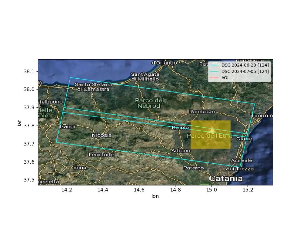
The selected bursts cover the area we are interested in, so everything looks fine up to now.
We are now ready to download the images, and to do so you need to create a free account at https://search.asf.alaska.edu/.
asf_username = 'username'
asf_password = '*****'

asf = ASF(asf_username, asf_password)

asf.download(DATADIR, BURSTS)

S1.download_orbits(DATADIR, S1.scan_slc(DATADIR))

# download Copernicus Global DEM 1 arc-second
Tiles().download_dem(AOI, filename=DEM)

# This is not needed for our analysis, but I keep it in case you need perform your own analysis.
Tiles().download_landmask(AOI, filename=LANDMASK).fillna(0).plot.imshow(cmap='binary_r')

# We use dask to perform multicore computing.

if 'client' in globals():
    client.close()
client = Client()
We can now load the downloaded data. Before using them, we need to preprocess them, because a single measurement is composed by multiple pictures, and we must stack them.
scenes = S1.scan_slc(DATADIR)
sbas = Stack(WORKDIR, drop_if_exists=True).set_scenes(scenes)
We will now crop the images to the AOI to reduce the computational effort.
sbas.compute_reframe(AOI)
We must now load the DEM model and the landmask, if used.
sbas.load_dem(DEM, AOI)

sbas.load_landmask(LANDMASK)

sbas.plot_scenes(AOI=AOI, dem=sbas.get_dem().where(sbas.get_landmask()), caption='Sentinel1 Landmasked Frame on DEM',
                 aspect='equal')
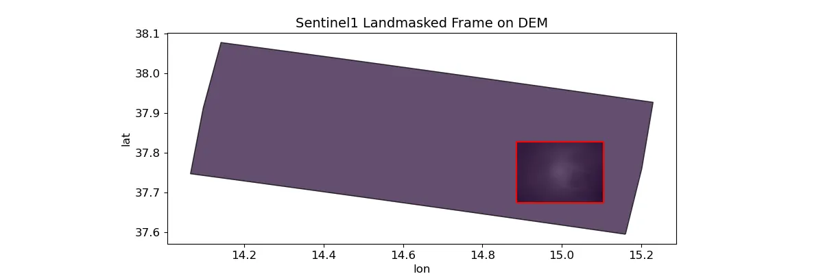
Since the two images cover a slightly different area because of the different position of the satellite, we must allign the images. Moreover, the measurements are not yet geocoded, so we must geocode them.
sbas.compute_align()

sbas.compute_geocode(45.)
Interferogram computation
We can now finally compute the interferogram, and we will keep the code as detailed as the original one.
# for a pair of scenes only two interferograms can be produced
# this one is selected for scenes sorted by the date in direct order
pairs = [sbas.to_dataframe().index]

# load radar topography
topo = sbas.get_topo()
# load Sentinel-1 data
data = sbas.open_data()
# Gaussian filtering 90m cut-off wavelength with multilooking 3x12 on Sentinel-1 intensity
intensity = sbas.multilooking(np.square(np.abs(data)), wavelength=90, coarsen=(3,12))
# calculate phase difference with topography correction
phase = sbas.phasediff(pairs, data, topo)
# Gaussian filtering 90m cut-off wavelength with multilooking
phase = sbas.multilooking(phase, wavelength=90, coarsen=(3,12))
# correlation on 3x12 multilooking data
corr = sbas.correlation(phase, intensity)
# Goldstein filter in 32 pixel patch size on square grid cells produced using 1:4 range multilooking
phase_goldstein = sbas.goldstein(phase, corr, 16)
# convert complex phase difference to interferogram
intf = sbas.interferogram(phase_goldstein)
# materialize for a single interferogram
tqdm_dask(result := dask.persist(intf[0], corr[0]), desc='Compute Phase and Correlation')
# unpack results
intf, corr = result

# geocode
intf_ll = sbas.ra2ll(intf)
corr_ll = sbas.ra2ll(corr)
dem = sbas.get_dem().interp_like(intf_ll).where(np.isfinite(intf_ll))
landmask_ll = sbas.get_landmask().interp_like(intf_ll)

sbas.plot_interferogram(intf_ll.where(landmask_ll), aspect='equal')
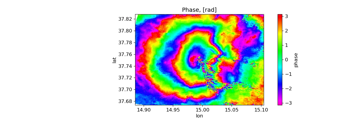
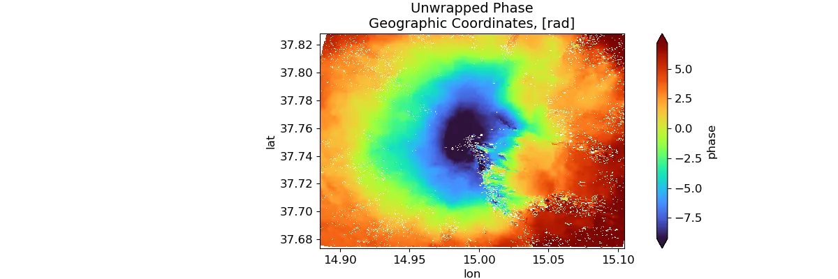
What we see in the above image is the phase difference, and since the phase is a periodic quantity, the phase difference is determined modulo $2 \pi.$ In order to translate it into a displacement, we must first unwrap it, and this is probably the hardest part of the analysis, from a computational point of view. PyGMTSAR relies on SNAPHU for this task, and this software uses complex analysis as well as the correlation between the two measurements to decide where there is a phase jump and where there is no jump.
Let us first of all plot the correlation
sbas.plot_correlation(corr_ll.where(landmask_ll), aspect='equal')
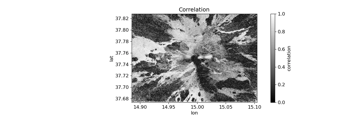
The correlation is almost zero in the south-east region of the volcano, probably due to some lavic flow. This makes the phase reconstruction less reliable. Fortunately, the low correlation region is bounded.
# mask low-coherence areas using threshold value 0.075
tqdm_dask(unwrap := sbas.unwrap_snaphu(intf.where(corr>=0.075), corr).persist(),
          desc='SNAPHU Unwrapping')
# apply simplest detrending
unwrap['phase'] = unwrap.phase - unwrap.phase.mean()

# geocode to geographic coordinates and crop empty borders
unwrap_ll = sbas.ra2ll(unwrap.phase)

sbas.plot_phase(unwrap_ll.where(landmask_ll), caption='Unwrapped Phase\nGeographic Coordinates, [rad]',
                quantile=[0.02, 0.98], aspect='equal')
We can finally compute the displacement (this is actually a multiplication)
# geocode to geographic coordinates and crop empty borders
los_disp_mm_ll = sbas.los_displacement_mm(unwrap_ll)

sbas.plot_displacement(los_disp_mm_ll.where(landmask_ll), caption='LOS Displacement\nGeographic Coordinates, [mm]',
                       quantile=[0.01, 0.99], aspect='equal')
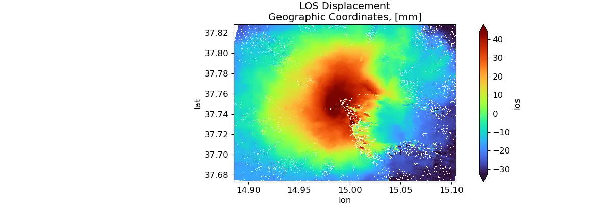
We can clearly see that the eruption caused a ground lift at the center of the volcano of roughly four centimeters.
Notice that the displacement is determined up to an overall additive constant which can be determined by applying some suitable boundary condition. The boundary condition is however difficult to determine due to the low correlation (and therefore low reliability) for large distances from the image center.
Conclusions
We have seen how to use PyMGSTAR to perform differential SAR interferometry. If you are interested in using this kind of technique, I recommend you taking some more advanced course on this topic, as both ESA and NASA have many courses on this topic, which can be really tricky.
Moreover, you should take a look at Alexey’s repo, since there are many ready-to-use notebooks, which will give show you the full capabilities of PyMGSTAR.