

OpenEO for SAR images
In the last post we discussed how to use OpenEO to access remote sensing data using the Sentinel 2 dataset. In this post we will use the same library to access the Sentinel 1 dataset, which is a Synthetic Aperture Radar mission which collected data from 2 satellites for many years. SAR is quite different from visible data, and as the name suggests, it is collected by a radar. This means that the light source is on the satellite, so it can collect data regardless on the sun position, keeping light intensity constant. Generally, SAR operates on frequencies much higher than the ones in the visible spectrum, so they do not interact with clouds, and allows for a great spatial resolution. These characteristics make SAR imaging a very interesting tool to monitor the Earth surface.
As you can imagine, there’s no free lunch, and we must pay a price in order to get the above advantages. One of the main disadvantages is that SAR images are really noisy, so you must put a lot of effort in image processing.
Oil spill detection
We will use the Sentinel-1 dataset to detect an oil spill in the Black Sea in 2024. A similar analysis can be found in this tutorial in the Copernicus documentation, but we will use xarray rather than Copernicus to perform the last steps of the analysis.
# Load the essentials
import openeo
import openeo.processes
import numpy as np

connection = openeo.connect("openeo.dataspace.copernicus.eu").authenticate_oidc()
connection.version_info()
'api': '1.2.0',
'backend': {'root_url': 'https://openeo.dataspace.copernicus.eu/openeo/1.2/',
'version': '0.66.0a5.dev20250619+2770',
'processing:software': {'geopyspark': 'n/a',
'geotrellis-extensions': '2.5.0_2.12-SNAPSHOT cba0c41',
'geotrellis-extensions-static': '2.5.0_2.12-SNAPSHOT cba0c41',
'openeo': '0.42.1',
'openeo-geopyspark': '0.66.0a5.dev20250619+2770',
'openeo_driver': '0.135.0a3.dev20250605+1169',
'openeo_udf': '1.0.0rc3.post1'}}}
bbox = [36.276855,44.742832,36.952515,45.197522]

def bbox_to_polygon(bbox):
    xmin = bbox[0]
    xmax = bbox[2]
    ymin = bbox[1]
    ymax = bbox[3]
    aoi = {
        "type": "Polygon",
        "coordinates": [
            [
                [xmin, ymax],
                [xmin, ymin],
                [xmax, ymin],
                [xmax, ymax],
                [xmin, ymax]
            ]
        ],
    }
    return aoi

aoi = bbox_to_polygon(bbox)

date_min = '2024-12-16'
date_max = '2024-12-25'

s1_image = connection.load_collection(
    "SENTINEL1_GRD",
    temporal_extent=[date_min, date_max],
    spatial_extent=aoi,
    bands=["VV"],
)

# We select the first available image
s1_image = s1_image.min_time()

# We want to get the total amount of reflected radiation, so we must use this method
s1_image = s1_image.sar_backscatter(coefficient="sigma0-ellipsoid")


# Moving to decibels, as the signal is quite noisy
s1_image = s1_image.apply(process=lambda data: 10 * openeo.processes.log(data, base=10))

# We can now save the image locally ans analyze it
s1_image.execute_batch(title="Oil Spill", outputfile="OilSpillBlackSea.nc")
0:00:13 Job 'j-2707301343334769a080b0f2ea48aca2': created (progress 0%)
0:00:18 Job 'j-2707301343334769a080b0f2ea48aca2': created (progress 0%)
0:00:25 Job 'j-2707301343334769a080b0f2ea48aca2': created (progress 0%)
0:00:33 Job 'j-2707301343334769a080b0f2ea48aca2': created (progress 0%)
0:00:43 Job 'j-2707301343334769a080b0f2ea48aca2': running (progress N/A)
0:00:55 Job 'j-2707301343334769a080b0f2ea48aca2': running (progress N/A)
0:01:10 Job 'j-2707301343334769a080b0f2ea48aca2': running (progress N/A)
0:01:30 Job 'j-2707301343334769a080b0f2ea48aca2': running (progress N/A)
0:01:54 Job 'j-2707301343334769a080b0f2ea48aca2': running (progress N/A)
0:02:24 Job 'j-2707301343334769a080b0f2ea48aca2': running (progress N/A)
0:03:01 Job 'j-2707301343334769a080b0f2ea48aca2': running (progress N/A)
0:03:48 Job 'j-2707301343334769a080b0f2ea48aca2': finished (progress 100%)
Obtaining and pre-processing the images was very easy, but not very interesting. Let us now move to the fun part.
Let us first of all open a new notebook 1
import matplotlib.pyplot as plt
import matplotlib
import xarray as xr
import pandas as pd
import geopandas as gpd
import matplotlib.patches as mpatches
from rasterio.plot import show, show_hist

oilspill = xr.load_dataset("./OilSpillBlackSea.nc")

fig, ax = plt.subplots()
show_hist(oilspill.VV.values, bins=80, ax=ax)
Let us now take a look at the data
fig, ax = plt.subplots(figsize=(9, 9))
show(oilspill.VV.values, transform=oilspill.rio.transform(), ax=ax)
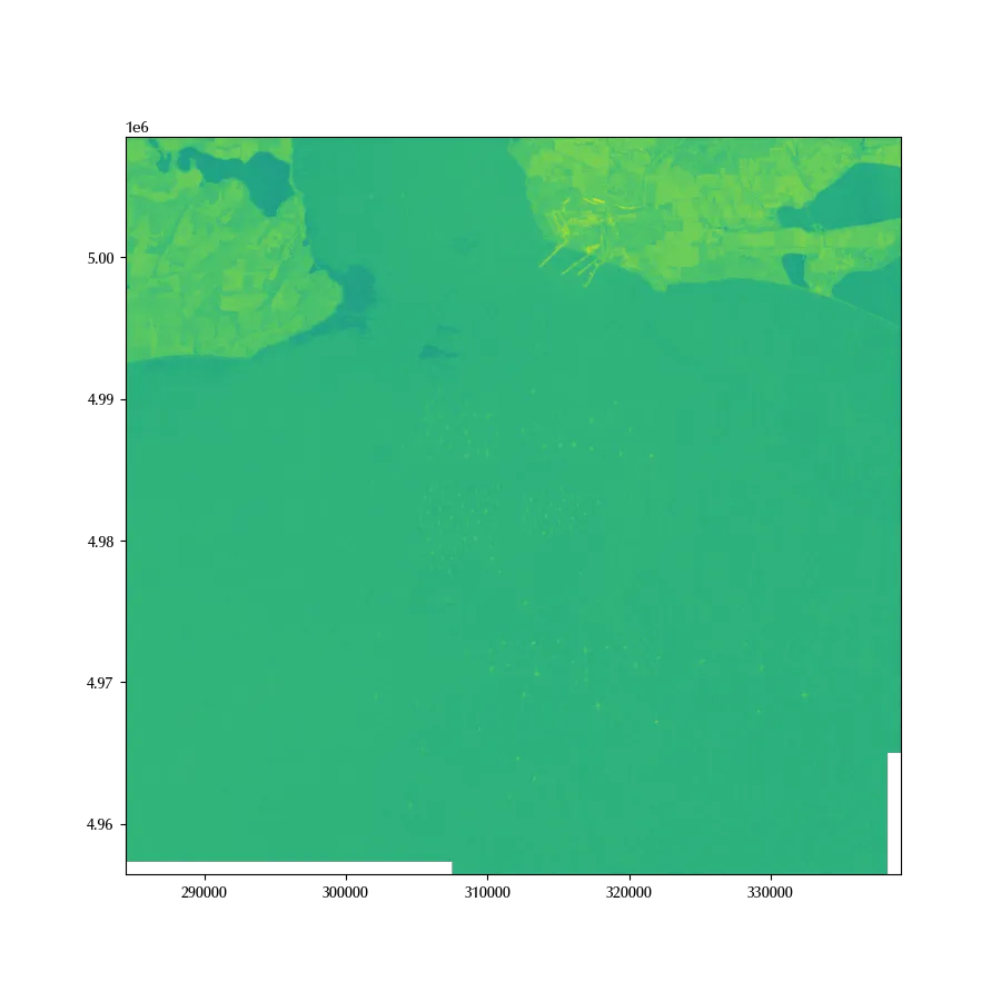
In the above figure, lighter pixels correspond to regions with higher reflectivity, while darker pictures are pixels where there is low reflection towards the satellite. A point might be darker either because the radiation is absorbd, or because the reflection is omnidirectional.
Let us now focus on the marine areas, where most of the sea have a green colour. Bright points correspond to ships, and we can see many of them. There are however two very dark regions, and they are regions where the oil dispersed.
Let us first of all crop the image onto the interesting regions. We do this for two reasons: the first one is due to the presence of NaN values, which are areas where the satellite could not collect enough reliable information. The second reason is simply that this will make our analysis faster, since processing large raster data can be quite computationally demanding
ds = oilspill.where(oilspill.x<315000, drop=True).where(oilspill.y>4.99e6, drop=True
                                                        ).dropna(dim='x').dropna(dim='y')
We will now perform a rolling median with a step equal to 5 in order to make the signal a little bit less noisy
ds_rolling = ds.VV.rolling(x=5, y=5).median()
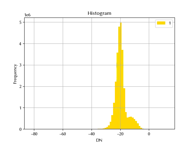
We are now ready to digitalize our data, and we will classify as “bright” points belonging to the right tail of the upper gaussian, while “dark” points. In order to keep things simple, we will (quite arbitrarily) choose -25 and -15 as threshold values respectively, simply by looking at the above histogram. We will leave to the reader the task to find an appropriate model to perform the classification.
cmap = matplotlib.colors.ListedColormap([(0, 0, 0, 0), 'purple'])

cmap1 = matplotlib.colors.ListedColormap([(0, 0, 0, 0), 'green'])

fig, ax = plt.subplots()
show(ds_rolling.values, transform=ds.rio.transform(), ax=ax, cmap='Greys')
show(
    (ds_rolling.values<-25),
    vmin=0,
    vmax=1,
    cmap=cmap,
    transform=ds.rio.transform(),
    ax=ax,
)

show(
    (ds_rolling.values>-15),
    vmin=0,
    vmax=1,
    cmap=cmap1,
    transform=ds.rio.transform(),
    ax=ax,
)
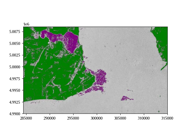
The above choice seems quite accurate, and both the oil spill and the ships have been correctly identified.
Conclusions
We have seen how to use SAR images to detect ships as well as oil spill, and we discussed advantages and disadvantages of SAR images over passive detection methods. If you are interested in this topic, I would recommend you to take a look at the many resources on this topic in order to understand the physical mechanism behind SAR imaging. As a good starting point I would recommend EdX Alaska-SAR course.
%load_ext watermark
%watermark -n -u -v -iv -w
Python implementation: CPython
Python version : 3.12.8
IPython version : 8.31.0
matplotlib: 3.10.1
rasterio : 1.4.3
xarray : 2025.1.1
Watermark: 2.5.0
-
This is my own way of working, as I prefer to be able and re-launch the entire analysis notebook on the downloaded images. ↩