

OpenEO 2: time series
The capabilities of OpenEO are not limited to the ones described in the previous post, as it allows us to perform complex analysis on the cloud, thanks to its API. We will show how to use it to monitor the time evolution of the vegetation status of the major parks in my own city, Turin. We will follow this tutorial on the Copernicus website. First of all, I downloaded the green urban areas file, named “aree verdi urbane”, in the webpage of the city.
import pandas as pd
import geopandas as gpd
import json
import openeo
import numpy as np
import seaborn as sns
from matplotlib import pyplot as plt
from scipy.signal import windows

gdf = gpd.read_file('/home/stippe/Downloads/torino_verde/verde_urbano/verde_urbano.dbf')

gdf.head()
| area | perimeter | giardini_ | giardini_i | cod | nome | pv | numero | gid | geometry | |
|---|---|---|---|---|---|---|---|---|---|---|
| 0 | 63357.7 | 1087.01 | 2 | 636 | 5 | PARCO PUBBLICO | 0 | 53136 | POLYGON ((404056.03125 5005447.5, 404222.1875 5005403.5, 404289 5005390.5, 404331.34375 5005366, 404297.15625 5005248.5, 404215.6875 5005274.5, 404199.375 5005224, 404199.375 5005185, 404191.25 5005177, 404178.21875 5005172, 403950.125 5005237, 403979.4375 5005297.5, 404031.5625 5005400, 404056.03125 5005447.5)) | |
| 1 | 9958.09 | 513.948 | 3 | 637 | 5 | PARCO PUBBLICO | 0 | 53137 | POLYGON ((396432.1875 5003903, 396452.875 5003903, 396453.78125 5003868, 396472.6875 5003868, 396487.96875 5003873.5, 396487.09375 5003891.5, 396497.875 5003890.5, 396506.875 5003926.5, 396531.1875 5003920, 396535.6875 5003892.5, 396533.875 5003865.5, 396531.1875 5003831, 396535.6875 5003802.5, 396430.375 5003795, 396432.1875 5003903)) | |
| 2 | 3491.65 | 252.427 | 4 | 683 | 5 | VERDE | 0 | 53138 | POLYGON ((394359.375 5001702, 394375.75 5001703.5, 394397.53125 5001690, 394401.625 5001612, 394359.375 5001612, 394359.375 5001702)) | |
| 3 | 9708.98 | 410.819 | 5 | 12 | 0 | Parco urbano | 0 | 53139 | POLYGON ((418021.3125 5001612, 418031.78125 5001613, 418033.65625 5001572, 418053.59375 5001524.5, 417928.3125 5001526.5, 417926.40625 5001614, 418021.3125 5001612)) | |
| 4 | 10220.2 | 496.126 | 6 | 13 | 0 | Parco urbano | 0 | 53140 | POLYGON ((415753.84375 5001383, 415789.0625 5001470, 415895.90625 5001453.5, 415893.5625 5001431, 415856 5001433.5, 415858.34375 5001371.5, 415870.09375 5001375, 415863.03125 5001364, 415872.4375 5001357, 415866.5625 5001343, 415753.84375 5001383)) |
gdf['area'].plot(kind='hist', bins=30)
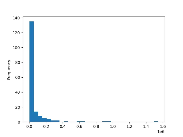
Most of the parks have an area below 100000 square meters, and we will limit our analysis to the largest.
gdf_filt = gdf[gdf['area']>3e5]
gdf_filt.explore()
We are now ready to prepare our job, and we will analyze the NDVI measurements. First of all, we must convert the dataset to a geojson into the ESPG 4326 projection.
fields = json.loads(
    gdf_filt.to_crs(4326).to_json()
)
We must now connect to the Copernicus dataspace and authenticate
openeo.client_version()
connection = openeo.connect(url="openeo.dataspace.copernicus.eu")
connection.authenticate_oidc()
As in the second part of the above example, we will compute the NDVI and mask the data using the cloud mask, so we will need the red, NIR and SCL bands. We will use the (rather robust) approach suggested in the tutorial, using a gaussian filter to create a larger cloud mask.
s2cube = connection.load_collection(
    "SENTINEL2_L2A",
    temporal_extent=["2022-01-01", "2025-06-01"],
    bands=["B04", "B08", "SCL"],
)

scl = s2cube.band("SCL")
mask = ~((scl == 4) | (scl == 5))


# 2D gaussian kernel
g = windows.gaussian(11, std=1.6)
kernel = np.outer(g, g)
kernel = kernel / kernel.sum()

# Morphological dilation of mask: convolution + threshold
mask = mask.apply_kernel(kernel)
mask = mask > 0.1

red = s2cube.band("B04")
nir = s2cube.band("B08")
ndvi = (nir - red) / (nir + red)

ndvi_masked = ndvi.mask(mask)
We can now compute the spatial average for each park
timeseries = ndvi_masked.aggregate_spatial(geometries=fields, reducer="mean")
job = timeseries.execute_batch(out_format="CSV", title="NDVI timeseries")
0:00:13 Job 'j-25061707203640dea32cddbfbd148f89': created (progress 0%)
0:00:18 Job 'j-25061707203640dea32cddbfbd148f89': created (progress 0%)
0:00:25 Job 'j-25061707203640dea32cddbfbd148f89': created (progress 0%)
0:00:33 Job 'j-25061707203640dea32cddbfbd148f89': created (progress 0%)
0:00:43 Job 'j-25061707203640dea32cddbfbd148f89': running (progress N/A)
0:00:56 Job 'j-25061707203640dea32cddbfbd148f89': running (progress N/A)
0:01:11 Job 'j-25061707203640dea32cddbfbd148f89': running (progress N/A)
0:01:31 Job 'j-25061707203640dea32cddbfbd148f89': running (progress N/A)
0:01:55 Job 'j-25061707203640dea32cddbfbd148f89': running (progress N/A)
0:02:25 Job 'j-25061707203640dea32cddbfbd148f89': running (progress N/A)
0:03:03 Job 'j-25061707203640dea32cddbfbd148f89': running (progress N/A)
0:03:49 Job 'j-25061707203640dea32cddbfbd148f89': running (progress N/A)
0:04:48 Job 'j-25061707203640dea32cddbfbd148f89': running (progress N/A)
0:05:48 Job 'j-25061707203640dea32cddbfbd148f89': running (progress N/A)
0:06:48 Job 'j-25061707203640dea32cddbfbd148f89': running (progress N/A)
0:07:49 Job 'j-25061707203640dea32cddbfbd148f89': running (progress N/A)
0:08:49 Job 'j-25061707203640dea32cddbfbd148f89': running (progress N/A)
0:09:50 Job 'j-25061707203640dea32cddbfbd148f89': finished (progress 100%)
After 10 minutes the job is finished, so we can now download and analyze the results.
job.get_results().download_file("timeseries-masked.csv")

df = pd.read_csv('timeseries-masked.csv')

df['date'] = pd.to_datetime(df['date'])

gdf1 = gdf_filt.copy()
gdf1['feature_index'] = range(len(gdf1))

fig, ax = plt.subplots(figsize=(9, 6))
sns.scatterplot(df_merged, x='date', y='band_unnamed', hue='nome', palette='Set2', ax=ax,
               alpha=0.8)
sns.move_legend(ax, "upper left", bbox_to_anchor=(1, 1))
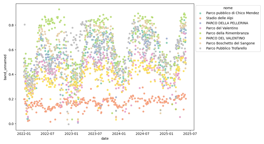
We can see a series which is much lower than the other ones, and this is a stadium, while the remaining parks are true parks.
There is of course a very large periodic component, since the photosynthesis processes are strongly seasonal.
It looks like there’s a small growing trend, and this is of course a good signal, but we should understand why this trend appears. Before drawing any conclusion, it would be wise to make sure that there is an explanation for this, and this is not some kind of artifact.
There is some possible outlier, probably due to some residual cloud, so we should take care of them if we want to perform a quantitative data analysis.
Conclusions
We have seen how to compute the NDVI time series for few city parks, and of course this approach can be immediately extended to precision agriculture and precision forestry, making the Copernicus data and its API invaluable.
%load_ext watermark

%watermark -n -u -v -iv -w
Python implementation: CPython
Python version : 3.12.8
IPython version : 8.31.0
matplotlib: 3.10.1
json : 2.0.9
seaborn : 0.13.2
numpy : 2.1.3
scipy : 1.15.2
geopandas : 1.0.1
pandas : 2.2.3
openeo : 0.40.0
Watermark: 2.5.0