

OpenEO
One of the main reasons GIS became popular is due to the possibility to access and process satellite and, generally, remote data. One of the best tools to do so is via OpenEO, a Python library that allows you to select and preprocess satellite data in an incredibly simple way. One of the main difficulties with remote sensors data is that you must process tons of different images in an analysis, and OpenEO has a backend that does that for you. This has two main advantages: it saves you a lot of time, and it avoids you a lot of errors, since the preprocessing backend is very robust and well tested.
OpenEO is an interface for many different providers, most of them require an account, and most of them need some payment subscription. The Copernicus free subscription, however, allows you to process a very large amount of data, so if you are a private user it’s unlikely that it doesn’t fit your needs. We will use OpenEO for landslide monitoring, as explained in this very well writen tutorial. If you are interested in using OpenEO, I strongly recommend you to look at all the examples in the above site.
Landslide monitoring via NDVI changes
The method proposed in the example is to look for abrupt vegetation losses to monitor landslides. This can be done in few very easy steps by using OpenEO, and we will do so on a large landslide reported on the Procida mount, close to Naples, on the 12th July 2024.
](/docs/assets/images/gis/openeo/ANSAprocida.jpg)
A picture of the landslide. Source ANSA.
Let us now start with the analysis
import openeo
import matplotlib
from matplotlib import pyplot as plt
import xarray as xr
from rasterio.plot import show
import rioxarray as rxr
import matplotlib as mpl
import matplotlib.colors
import matplotlib.patches as mpatches
import numpy as np
import pandas as pd
import geopandas as gpd

conn = "openeo.dataspace.copernicus.eu"

# Having the coastal boundaries will help us in avoiding false signals
gdf_it = gpd.read_file('/home/stippe/Downloads/italy/gadm41_ITA_0.dbf')

# First of all, we connect to the API
connection = openeo.connect(conn).authenticate_oidc()
The above message comes since I already performed the login in the past. Let us look at the available collections
connection.list_collection_ids()
'SENTINEL3_SLSTR',
'SENTINEL_5P_L2',
'COPERNICUS_VEGETATION_PHENOLOGY_PRODUCTIVITY_10M_SEASON1',
'COPERNICUS_VEGETATION_PHENOLOGY_PRODUCTIVITY_10M_SEASON2',
'COPERNICUS_PLANT_PHENOLOGY_INDEX',
'ESA_WORLDCOVER_10M_2020_V1',
'ESA_WORLDCOVER_10M_2021_V2',
'COPERNICUS_VEGETATION_INDICES',
'SENTINEL2_L1C',
'SENTINEL2_L2A',
'SENTINEL1_GRD',
'COPERNICUS_30',
'LANDSAT8_L2',
'SENTINEL3_SYN_L2_SYN',
'SENTINEL3_SLSTR_L2_LST',
'SENTINEL1_GLOBAL_MOSAICS',
'SENTINEL3_OLCI_L2_LAND',
'SENTINEL3_OLCI_L2_WATER',
'SENTINEL3_SYN_L2_AOD']
As you can see, there’s a large variety of collections. We will use the Sentinel 2 layer 2A data.
df_bands = pd.DataFrame.from_records(connection.describe_collection('SENTINEL2_L2A')['summaries']['eo:bands'])
df_bands[df_bands['name'].astype(str).str.startswith("B")]
| aliases | center_wavelength | common_name | full_width_half_max | gsd | name | offset | scale | type | unit | |
|---|---|---|---|---|---|---|---|---|---|---|
| 0 | [‘IMG_DATA_Band_B01_60m_Tile1_Data’] | 0.4427 | coastal | 0.021 | 60 | B01 | 0 | 0.0001 | int16 | 1 |
| 1 | [‘IMG_DATA_Band_B02_10m_Tile1_Data’] | 0.4924 | blue | 0.066 | 10 | B02 | 0 | 0.0001 | int16 | 1 |
| 2 | [‘IMG_DATA_Band_B03_10m_Tile1_Data’] | 0.5598 | green | 0.036 | 10 | B03 | 0 | 0.0001 | int16 | 1 |
| 3 | [‘IMG_DATA_Band_B04_10m_Tile1_Data’] | 0.6646 | red | 0.031 | 10 | B04 | 0 | 0.0001 | int16 | 1 |
| 4 | [‘IMG_DATA_Band_B05_20m_Tile1_Data’] | 0.7041 | nan | 0.015 | 20 | B05 | 0 | 0.0001 | int16 | 1 |
| 5 | [‘IMG_DATA_Band_B06_20m_Tile1_Data’] | 0.7405 | nan | 0.015 | 20 | B06 | 0 | 0.0001 | int16 | 1 |
| 6 | [‘IMG_DATA_Band_B07_20m_Tile1_Data’] | 0.7828 | nan | 0.02 | 20 | B07 | 0 | 0.0001 | int16 | 1 |
| 7 | [‘IMG_DATA_Band_B08_10m_Tile1_Data’] | 0.8328 | nir | 0.106 | 10 | B08 | 0 | 0.0001 | int16 | 1 |
| 8 | [‘IMG_DATA_Band_B8A_20m_Tile1_Data’] | 0.8647 | nir08 | 0.021 | 20 | B8A | 0 | 0.0001 | int16 | 1 |
| 9 | [‘IMG_DATA_Band_B09_60m_Tile1_Data’] | 0.9451 | nir09 | 0.02 | 60 | B09 | 0 | 0.0001 | int16 | 1 |
| 10 | [‘IMG_DATA_Band_B11_20m_Tile1_Data’] | 1.6137 | swir16 | 0.091 | 20 | B11 | 0 | 0.0001 | int16 | 1 |
| 11 | [‘IMG_DATA_Band_B12_20m_Tile1_Data’] | 2.2024 | swir22 | 0.175 | 20 | B12 | 0 | 0.0001 | int16 | 1 |
In the above table, we have the entire list of available bands. In order to calculate the NDVI, we need the Near infrared (NIR) and the red. From http://bboxfinder.com I got the bounding box of the region we are interested in.
bbox = {
    'west': 14.027824,
    'south': 40.776252,
    'east': 14.093914,
    'north': 40.818096
}
Since the event happened on the 12th of July 2024, we will look for data one month before and one month after the event, and we will average over the entire month before/after.
range_pre=["2024-06-11", "2024-07-11"]
range_post=["2024-07-13", "2024-08-13"]
max_cloud = 40
We choose a maximum cloud fraction of $0.4$, and we are now ready to perform the analysis.
# We first collect all the relevant images
s2pre = connection.load_collection(
    "SENTINEL2_L2A",
    spatial_extent=bbox,
    temporal_extent=range_pre,
    bands=["B04", "B08"],
    max_cloud_cover=30,
)

# We then calculate the ndvi for each one and average over the period
prendvi = s2pre.ndvi().mean_time()

# We now perform the same operations for the second set of images

s2post = connection.load_collection(
    "SENTINEL2_L2A",
    spatial_extent=bbox,
    temporal_extent=range_post,
    bands=["B04", "B08"],
    max_cloud_cover=30,
)

postndvi = s2post.ndvi().mean_time()

diff = postndvi - prendvi

diff
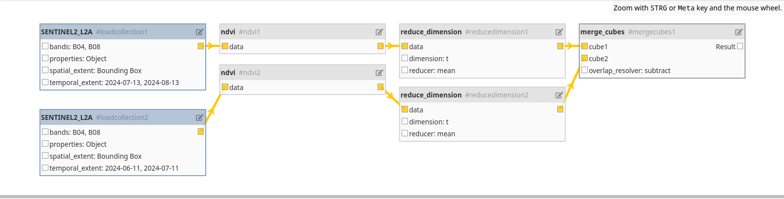
Not a single operation has been performed up to now, the entire set of operations was only an abstraction. We will now ask to download the result, and OpenEO will perform the entire analysis for us.
diff.download("NDVIDiffProcida.tiff")
We are now able to visualize the result. We will perform a visualization very similar to the one used in the above tutorial, with the only difference that we will use xarray instead of rasterio and that we will mask the result within the coastal lines.
gdf_pts = gpd.GeoDataFrame(geometry=gpd.points_from_xy([14.07252051], [40.78744825]),
                           data={'Label': ['Miliscola'], 'Color': ['green']}, crs=4326)

xy_ann = (gdf_pts.to_crs(clipped.rio.crs)['geometry'].values.x[0],
      gdf_pts.to_crs(clipped.rio.crs)['geometry'].values.y[0])

xy_ann = np.array(xy_ann) - np.array([1.5e3, 2e2])

rxarr = rxr.open_rasterio("NDVIDiffProcida.tiff")
clipped = rxarr .rio.clip(gdf_it.to_crs(rxarr.rio.crs)['geometry'])

value = clipped.sel(band=1).values
cmap = matplotlib.colors.ListedColormap(["lightgrey", "red"])
fig, ax = plt.subplots()
im = show(
    ((value < -0.48) & (value > -1)),
    vmin=0,
    vmax=1,
    cmap=cmap,
    transform=clipped.rio.transform(),
    ax=ax,
)
values = ["Absence", "Presence"]
colors = ["lightgrey", "red"]
ax.set_title("Detected Landslide Area")
ax.set_xlabel("X Coordinates")
ax.set_ylabel("Y Coordinates")
xlim = ax.get_xlim()
ylim = ax.get_ylim()
gdf_it.to_crs(img.crs).boundary.plot(ax=ax, color='k')
gdf_pts.to_crs(clipped.rio.crs).plot(ax=ax, color='green')
ax.annotate('REPORTED LOCATION', xy=xy_ann, color='k')
ax.set_xlim(xlim)
ax.set_ylim(ylim)
patches = [
    mpatches.Patch(color=colors[i], label="Landslide {l}".format(l=values[i]))
    for i in range(len(values))
]
fig.legend(handles=patches, bbox_to_anchor=(0.53, 0.27), loc=1)
fig.tight_layout()
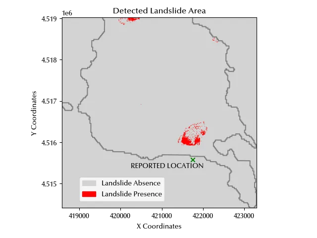
This website provides a more precise location of the landslide, and the ISPRA website provides at the above link the coordinates of the corresponding beach. The above coordinates have been shown in green in our plot, and the beach is very close to the NDVI index variation.
Conclusions
OpenEO gives you the opportunity to use a huge collection of data to perform your analysis, and it also gives you a simple interface to perform the analysis.
%load_ext watermark
%watermark -n -u -v -iv -w
Python implementation: CPython
Python version : 3.12.8
IPython version : 8.31.0
rioxarray : 0.18.2
rasterio : 1.4.3
pandas : 2.2.3
xarray : 2025.1.1
geopandas : 1.0.1
numpy : 2.1.3
matplotlib: 3.10.1
openeo : 0.40.0
Watermark: 2.5.0