

Digital Elevation Models
Digital Elevation Models (DEMs) are the larger family of a set of models encoding geographic information. DEMs can be divided into two families, depending on the information provided:
- Digital Terrain Models (DTMs) encode information regarding the ground
- Digital Surface Models (DSMs) encode information regarding all the objects on the ground, such as buildings or vegetation.
DEMs can be stored into two different formats:
- GRID DEMs store information into an equally spaced grid
- Triangular Irregular Network (TIN) DEMs store information into an irregular grid
Which one you should choose for your project depends on your needs but, mostly, on the availability, since you will rarely use your own DEM, unless you are a specialist on the topic. Needless to say that DEMs find applications in a variety of topics, from flood analysis to hiking maps, so it’s crucial to understand this topic, and I recommend you to have a deeper dive into this topic.
Here we will only give an overview to the most common kinds of information you can extract from a DEM, but we will not cover another fundamental topic, namely how to perform a proper uncertainty assessment.
Choosing the most appropriate DEM
The first choice you must perform is, of course, the DEM you want to use, and as usual this both depends on your needs and on what DEMs are available for your region of interest. You must of course choose between using a DTM or a DSM and between a grid or a TIN model, but there are many other possible relevant factors such as the resolution (both horizontal and vertical) or the age of your DEM.
A valuable website which freely distributes high quality DEMs is Open Topography, and you can easily connect it to QGIS via its plugin.
We won’t follow this strategy here, and we will use the Python package
elevation to obtain the data.
import xarray as xr
import rioxarray as rxr
import xrspatial as xrs
import elevation
from matplotlib import pyplot as plt

elevation.clip(bounds=(12.35, 41.8, 12.65, 42), output='Rome-DEM.tif')
make: Nothing to be done for 'download'.
make: Leaving directory '/home/user/.cache/elevation/SRTM1'
make: Entering directory '/home/user/.cache/elevation/SRTM1'
make: Nothing to be done for 'all'.
make: Leaving directory '/home/user/.cache/elevation/SRTM1'
make: Entering directory '/home/user/.cache/elevation/SRTM1'
cp SRTM1.vrt SRTM1.898269efd68743d6a7674b41e0d45d54.vrt
make: Leaving directory '/home/user/.cache/elevation/SRTM1'
make: Entering directory '/home/user/.cache/elevation/SRTM1'
gdal_translate -q -co TILED=YES -co COMPRESS=DEFLATE -co ZLEVEL=9 -co PREDICTOR=2 -projwin 12.35 42.0 12.65 41.8 SRTM1.898269efd68743d6a7674b41e0d45d54.vrt Rome-DEM.tif
rm -f SRTM1.898269efd68743d6a7674b41e0d45d54.vrt
make: Leaving directory '/home/user/.cache/elevation/SRTM1'
In my case, this is not the first time I ran this code, so we get a lot of “Nothing to be done”, but in your case the output might differ. Let us now take a look at our data. If you are running your code in a Linux OS (as I hope you are doing ;)), you will find the data in the /home/$USER/.cache/elevation folder.
ds_elev_latlon = rxr.open_rasterio('/home/stippe/.cache/elevation/SRTM1/Rome-DEM.tif')

fig, ax = plt.subplots()
ds_elev_latlon.sel(band=1).plot(cmap='gist_earth', ax=ax)
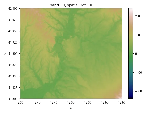
Here it comes the first issue, which is the CRS.
print(ds_elev_latlon.rio.crs)
This is an unprojected CRS, and it’s not appropriate for any manipulation involving distance quantities. As we previously stated, unless necessary, it’s better to avoid raster reprojections, since this procedure might introduce errors. If you can use a DEM which comes with a projected CRS in your analysis, you should probably consider using it rather than introducing additional sources of errors due to the reprojection. There are many DEMs online with a high resolution and which are already defined on a projected CRS, and by asking around or googling you might find what you need. Let us now reproject our DSM onto a more appropriate CRS. We will use the UTM 32 N projection, which has EPSG code 32632.
ds_elev_full = ds_elev_latlon.rio.reproject("EPSG:32632", nodata=-9999)
This however introduces nans into the grid, which are expressed as -9999, as specified into the above code.
fig, ax = plt.subplots()
ds_elev_full.sel(band=1).plot(cmap='gist_earth', ax=ax)
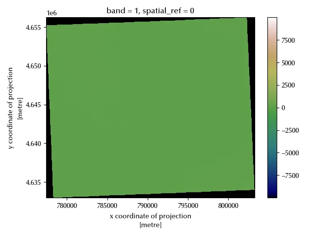
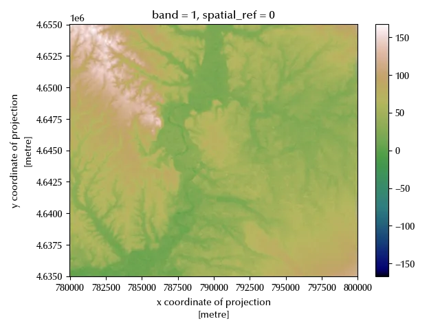
We must now take care of the null values, so we will clip the data.
bbox = [780000, 4635000, 800000, 4655000]

geometries = [
    {
        'type': 'Polygon',
        'coordinates': [[
            [bbox[0], bbox[1]],
            [bbox[0], bbox[3]],
            [bbox[2], bbox[3]],
            [bbox[2], bbox[1]],
            [bbox[0], bbox[1]],
        ]]
    }
]

ds_elev = ds_elev_full.rio.clip(geometries)

fig, ax = plt.subplots()
ds_elev.sel(band=1).plot(cmap='gist_earth', ax=ax)
DEM applications
We will now show how to extract some of the most relevant kind of products from a DEM:
- curve levels 1
- slope/aspect
- curvature
- viewshed
- hillshade
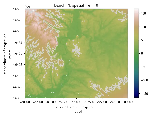
Curve levels can be easily plotted, either with matplotlib or with xarray, while obtaining the curve level coordinates needs a some more effort. It is however more likely that you only need to plot them, so we will only show how to perform this task.
fig, ax = plt.subplots()
ds_elev.sel(band=1).plot(cmap='gist_earth', ax=ax)
xr.plot.contour(ds_elev.sel(band=1), vmin=0, vmax=150, levels=3, ax=ax, colors='lightgray')
fig.tight_layout()
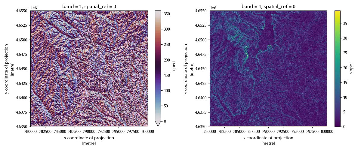
Another common kind of information one want to derive from a DEM is the one regarding the steepness of the terrain, and this information can be translated into two features:
- the aspect, which is the steepest direction at a given point.
- the slope, namely the magnitude of the gradient in aspect direction at a given point
Slope is generally expressed either in percentage or in degrees, and this quantity is meaningless in flat regions, while the aspect is expressed in degrees with respect to the North direction.
fig, ax = plt.subplots(ncols=2, figsize=(12, 5))
xrs.aspect(ds_elev.sel(band=1)).plot(cmap='twilight', ax=ax[0], vmin=0, vmax=360)
xrs.slope(ds_elev.sel(band=1)).plot(cmap='viridis', ax=ax[1])
fig.tight_layout()
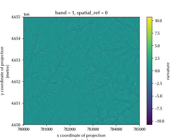
When you perform a landslide risk assessment, one of the core risk factors is generally the land curvature, since a convex terrain has more chances to undergo to a landslide rather than a concave one. We can easily obtain this information as follows
fig, ax = plt.subplots()
xrs.curvature(ds_elev.sel(band=1)).plot(cmap='viridis', ax=ax)
ax.set_xlim([780000, 785000])
ax.set_ylim([4650000, 4655000])
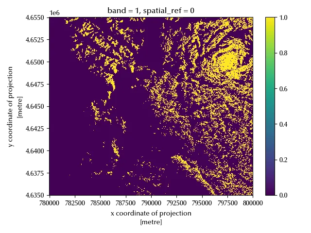
Viewshed analysis aims to determine what can or cannot be seen from a given point. Let us assume you want to place an antenna to improve the mobile coverage of a region, in this case you will likely want to maximize the viewshed in the uncovered area. If we want to place a 50 m antenna at x=797500 and y=4650000, as an example, we could determine the viewshed region as follows
vs = xrs.viewshed(ds_elev.sel(band=1), x=797500, y=4650000, observer_elev=50)
msk = vs>=0

fig, ax = plt.subplots()
msk.plot(cmap='viridis', ax=ax)
fig.tight_layout()
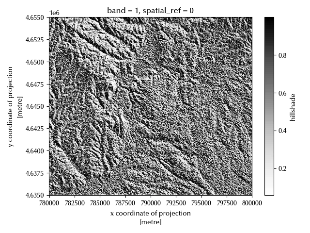
Hillshade is finally very important in map drawing, and this process emulates the amount of light which every point receives from a given light source.
fig, ax = plt.subplots()
xrs.hillshade(ds_elev.sel(band=1)).plot(ax=ax, cmap='Greys')
fig.tight_layout()
Conclusions
DEM analysis is a core part of many GIS applications, but performing a proper DEM analysis both requires a strong theoretical background and good tools. Here we have seen how to use Python to analyze DEMS.
%load_ext watermark
%watermark -n -u -v -iv -w
Python implementation: CPython
Python version : 3.12.8
IPython version : 8.31.0
numpy : 2.1.3
elevation : 1.1.3
xarray : 2025.1.1
matplotlib: 3.10.1
xrspatial : 0.4.0
rioxarray : 0.18.2
rasterio : 1.4.3
Watermark: 2.5.0
-
This kind of product is better extracted from a TIN dataset rather than from a grid one. Nonetheless, we will show how to get this kind of product. ↩