

Open Street Map services
Everybody knows Google Maps, and almost everybody uses it. Unfortunately, very few know that there exists an open alternative, and this alternative can be easily used within Python. In this post we will discuss OSMnx, a Python library that allows you to interrogate the OSM services. OSMnx comes with NetworkX, a powerful library built to manipulate networks, and this allows you to easily calculate routes between points.
OSMnx
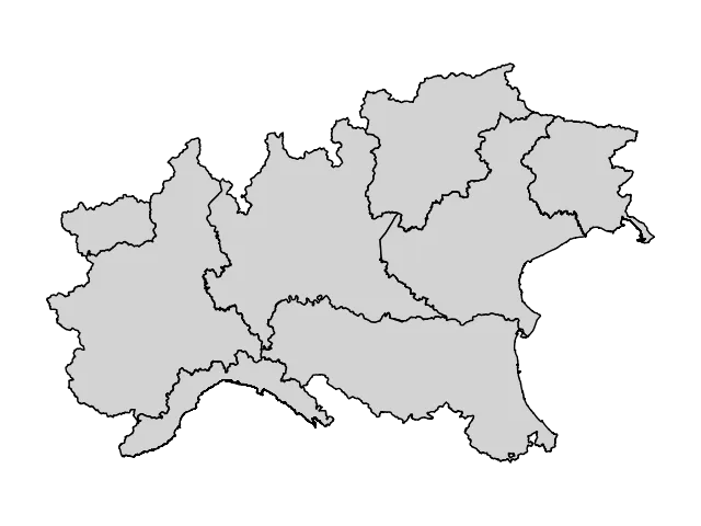
Let us start our tour in the OSMnx capabilities. We can easily get the boundaries of any location, from city neighborhoods to continents.
import numpy as np
import osmnx as ox
import networkx as nx
import pandas as pd
import geopandas as gpd
import matplotlib as mpl
from matplotlib import pyplot as plt

# These are the italian names of some region in north Itay

place_names = ["Piemonte", "Lombardia", "Liguria", "Val d'Aosta", "Trentino Alto Adige", "Veneto", "Friuli Venezia Giulia",
              "Emilia Romagna"]

gdf = ox.geocode_to_gdf(place_names)

fig, ax = plt.subplots()
gdf.plot(fc="lightgray", ec="black", ax=ax)
ax.axis("off")
fig.tight_layout()
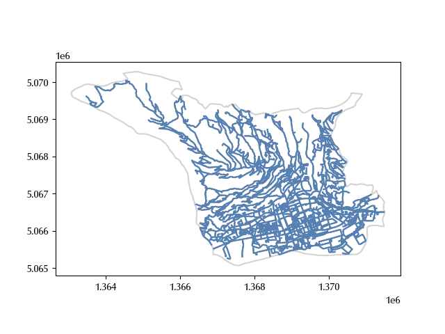
We can also download the walking route for a city.
# Let us first download the polygon for Aosta, a city in north Italy
aosta = ox.geocode_to_gdf("Aosta, Italy")

polygon = aosta["geometry"].iloc[0]

# We can now download the walking route for the corresponding polygon

G = ox.graph_from_polygon(polygon, network_type="walk")

# graphs are great for mathematical manipulation, but for GIS tasks it's better do separate them
# into nodes, which are points, and edges, which are lines

nodes = ox.graph_to_gdfs(G, nodes=True, node_geometry=True, edges = False).to_crs(crs = 3003)
edges = ox.graph_to_gdfs(G, nodes=False, edges =  True, fill_edge_geometry=True).to_crs(crs = 3003)

fig, ax = plt.subplots()
aosta.to_crs(3003).boundary.plot(ax=ax, color='lightgray')
edges.plot(ax=ax)
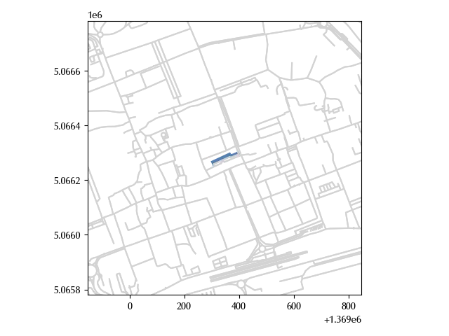
We can also retrieve building’s footprints, let us see this for the Aosta major building.
addr = "Municipio di Aosta, Italy"

geo = gpd.tools.geocode([addr], provider='nominatim', user_agent='autogis_xx', timeout=4)

tags = {'building': True} # would return all building footprints in the area
center_point = (geo['geometry'].y.iloc[0], geo['geometry'].x.iloc[0])

a = ox.features_from_point(center_point, tags, dist=20)

fig, ax = plt.subplots()
edges.plot(ax=ax, color='lightgray')
a.to_crs(edges.crs).plot(ax=ax)
ax.set_xlim([a.to_crs(edges.crs)['geometry'].centroid.x.iloc[0]-500,
             a.to_crs(edges.crs)['geometry'].centroid.x.iloc[0]+500])
ax.set_ylim([a.to_crs(edges.crs)['geometry'].centroid.y.iloc[0]-500,
             a.to_crs(edges.crs)['geometry'].centroid.y.iloc[0]+500])
fig.tight_layout()
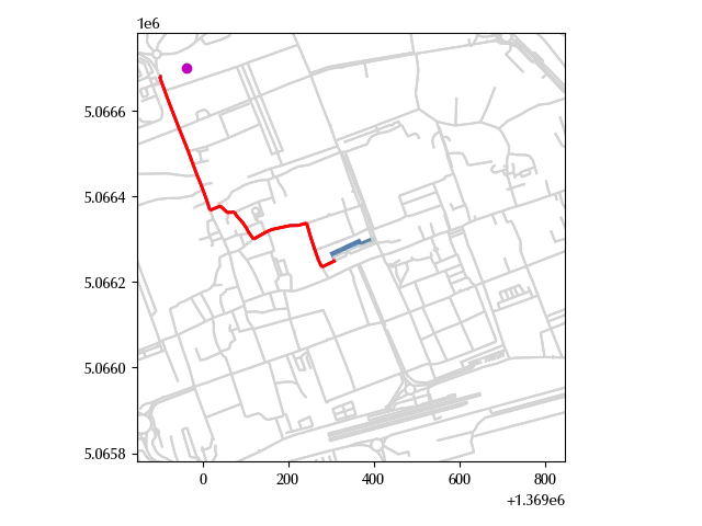
We can finally calculate the shortest path between two locations. Let us first search for the Aosta hospital
addr1 = "Ospedale di Aosta, Italy"
geo1 = geocode([addr1], provider='nominatim', user_agent='autogis_xx', timeout=4)
center_point1 = (geo1['geometry'].y.iloc[0], geo1['geometry'].x.iloc[0])

g1 = gpd.GeoDataFrame(geometry=gpd.points_from_xy([geo1['geometry'].x.iloc[0]], [geo1['geometry'].y.iloc[0]]),
                     crs=4326)
We can now calculate the shortest path from the hospital to the major building. We will first find the nearest node to the two locations, and then find the shortest path between the nodes.
start_node = ox.distance.nearest_nodes(G, geo1['geometry'].x.iloc[0], geo1['geometry'].y.iloc[0])
end_node = ox.distance.nearest_nodes(G, geo['geometry'].x.iloc[0], geo['geometry'].y.iloc[0])

route_nodes = ox.routing.shortest_path(G, start_node, end_node, weight="length")

G1 = G.subgraph(route_nodes)

nodes1 = ox.graph_to_gdfs(G1, nodes=True, node_geometry=True, edges = False).to_crs(crs = 3003)
edges1 = ox.graph_to_gdfs(G1, nodes=False, edges =  True, fill_edge_geometry=True).to_crs(crs = 3003)

fig, ax = plt.subplots()
edges.plot(ax=ax, color='lightgray')
edges1.plot(ax=ax, color='r', lw=2)
a.to_crs(edges.crs).plot(ax=ax)
g1.to_crs(edges.crs).plot(ax=ax, color='m')
ax.set_xlim([a.to_crs(edges.crs)['geometry'].centroid.x.iloc[0]-500,
             a.to_crs(edges.crs)['geometry'].centroid.x.iloc[0]+500])
ax.set_ylim([a.to_crs(edges.crs)['geometry'].centroid.y.iloc[0]-500,
             a.to_crs(edges.crs)['geometry'].centroid.y.iloc[0]+500])
fig.tight_layout()
Conclusions
Thanks to Open Street Map and NetworkX you can easily retrieve and manipulate a huge variety of geographic information, from streets to buildings.
%load_ext watermark
%watermark -n -u -v -iv -w
Python implementation: CPython
Python version : 3.12.8
IPython version : 8.31.0
pandas : 2.2.3
osmnx : 2.0.0
networkx : 3.4.2
numpy : 2.1.3
matplotlib: 3.10.1
geopandas : 1.0.1
Watermark: 2.5.0