

Open Web Consortium standards
In the last decades GIS became a relevant topic for most institutions, and the development of a common way to share GIS files became a hot topic. This is why the Open Web Consortium developed a set of standards to share GIS files. Here we will discuss the Python implementations of clients to read these files.
Web Feature Services
WFSs are services which allows you to get vector data. They are web service, and normally the response type is either geojson or xml.
# Load python libraries
from owslib.wcs import WebCoverageService
from owslib.wms import WebMapService
from owslib.wfs import WebFeatureService
import numpy as np
import rioxarray as rxr
import xarray as xr
import rasterio as rio
from rasterio.plot import show, show_hist
import seaborn as sns
from matplotlib import pyplot as plt
import pandas as pd
import geopandas as gpd
import geojson
import geojson

wfs_url = 'http://servizigis.regione.emilia-romagna.it/wfs/uso_del_suolo?request=GetCapabilities&service=WFS'
wms_url = 'http://servizigis.regione.emilia-romagna.it/wms/sfumo_altimetrico5x5?service=WMS&version=1.3.0&request=GetCapabilities'

wfs = WebFeatureService(wfs_url, version='2.0.0')

list(wfs.contents)
'portale_uso_del_suolo:_994_uso_suolo_ed2021',
'portale_uso_del_suolo:_003_uso_suolo_ed2021',
'portale_uso_del_suolo:_008_uso_suolo_ed2018',
'portale_uso_del_suolo:_014_uso_suolo_ed2018',
'portale_uso_del_suolo:_017_uso_suolo_ed2020',
'portale_uso_del_suolo:_020_uso_suolo_ed2023',
'portale_uso_del_suolo:_853_uso_suolo_storico_punti',
'portale_uso_del_suolo:_853_uso_suolo_storico_poligoni',
'portale_uso_del_suolo:_976_uso_suolo_ed2011',
'portale_uso_del_suolo:_994_uso_suolo_ed2015',
'portale_uso_del_suolo:_003_uso_suolo_ed2011',
'portale_uso_del_suolo:_008_uso_suolo_ed2011',
'portale_uso_del_suolo:_011_uso_suolo_ed2013']
The above output contains all the possible layers which can be downloaded. We will use the first one. Let us now see the available CRS for this layer.
wfs_sel = 'portale_uso_del_suolo:_976_78_uso_del_suolo_ed2024'

sorted(wfs[wfs_sel].crsOptions)
There’s only one available CRS. Let us now see the bounding box.
list(wfs.contents[wfs_sel].boundingBox)
There’s a first small issue here: the bounding box is expressed in a different CRS from the one available, so before sending the request we must convert it. We will not use the entire bounding box, since the request would go in timeout for that amount of data.
bbx_latlon = (11.479340,44.477858,11.585834, 44.562099 )

gdf_tmp = gpd.GeoDataFrame(geometry=gpd.points_from_xy(bbx_latlon[0:4:2], bbx_latlon[1:5:2]),
    crs=4326).to_crs(25832)

wfs_resp = wfs.getfeature(typename=wfs_sel, bbox=bbx, srsname=sorted(wfs[wfs_sel].crsOptions)[0])

wfs_val = wfs_resp.read()

wfs_val[:39]
The output type is xml. We will store it into an xml file and read the file with geopandas.
with open('geotmp.xml', 'wb') as f:
    f.write(wfs_val)
gdf = gpd.read_file('geotmp.xml')

gdf.columns
'COD_TOT', 'DESCR', 'HECTARES', 'SHAPE.AREA', 'SHAPE.LEN', 'geometry'],
dtype='object')
We will only keep a subset of the dataframe
relev = ['Boschi planiziari a prevalenza di farnie e frassini',
       'Boscaglie ruderali', 'Boschi a prevalenza di salici e pioppi',
       'Frutteti', 'Altre colture da legno', 'Pioppeti colturali',
       'Vigneti', 'Colture temporanee associate a colture permanenti',
        'Aree incolte urbane',
       'Sistemi colturali e particellari complessi', 'Parchi']

fig, ax = plt.subplots()
gdf_red.plot(ax=ax)
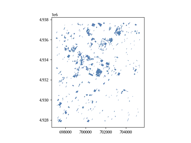
The relevant information is localized, and we will use the above limit for our second request
minvals = [696000, 4.926e6]
maxvals = [706000, 4.939e6]
deltax = maxvals[0]-minvals[0]
deltay = maxvals[1]-minvals[1]

deltaratio = deltay/deltax
deltaratio
Web Map Services
We can now proceed and download the elevation data
wms = WebMapService(wms_url, version='1.3.0')

wms.contents.keys()
wms_sel = 'Sfumo_Altimetrico5x5'

'EPSG:25832' in wms[wms_sel].crsOptions
Our initial CRS is available for the WMS, and this makes our life a little bit simpler. Let us now check if we can download a tif file.
wms.getOperationByName('GetMap').formatOptions
'image/png',
'image/png24',
'image/png32',
'image/bmp',
'image/gif',
'image/jpeg',
'image/svg',
'image/bil']
img = wms.getmap(
    layers=[wms_sel],
    size=[3000, 2000],
    srs='EPSG:25832',
    bbox=[minvals[0], minvals[1], maxvals[0], maxvals[1]],
    format="image/tiff")

with open('er.tif', "wb") as f:
    f.write(img.read())

data = rxr.open_rasterio('er.tif')

fig, ax = plt.subplots()
gdf_red.plot(ax=ax)
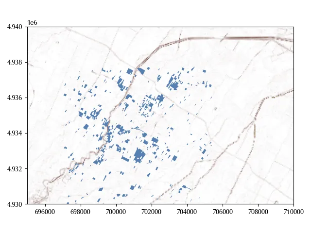
show(data.values, ax=ax, transform=data.rio.transform(), cmap='terrain')

ax.set_xlim([695000, 710000])
ax.set_ylim([4.93e6, 4.94e6])
fig.tight_layout()
Conclusion
We discussed two of the most popular ways to share GIS files,
namely WFS and WMS, and we have seen how to use owslib
to connect to WFS and WMS servers.
Many more functions are available, and you should
check the owslib page
to take a tour across all the functionalities that this library
provides.