

Map design
We already discussed how to show data in the dataviz section, here we will put the above topic in the geographic context.
If designing a good data visualization can be hard, map design can be harder, and this is one of the reasons why you should not use maps unless you need so.
We will do so for the dataset provided in this article which can be downloaded at this link.
import numpy as np
import pandas as pd
import geopandas as gpd
from matplotlib import pyplot as plt
import contextily as cx
import pyproj
from matplotlib_scalebar.scalebar import ScaleBar
from matplotlib_map_utils.core.north_arrow import NorthArrow, north_arrow
from matplotlib_map_utils.core.scale_bar import scale_bar

df = pd.read_csv('oo_404222.csv')

df.head()
| ID | CellCode | biogeographical_region | X | Y | |
|---|---|---|---|---|---|
| 0 | 1 | 10kmE587N749 | Outside | 5875000 | 7495000 |
| 1 | 2 | 10kmE588N749 | Outside | 5885000 | 7495000 |
| 2 | 3 | 10kmE589N749 | Outside | 5895000 | 7495000 |
| 3 | 4 | 10kmE590N749 | Outside | 5905000 | 7495000 |
| 4 | 5 | 10kmE591N749 | Outside | 5915000 | 7495000 |
The dataset provides, for each EU standard grid square, the corresponding biogeographical region.
In order to convert it into a geodataframe, we must first download the EU standard 10 km grid shapefile, and this can be done from this link.
gdf_base = gpd.read_file('europe_10km.dbf')

gdf_start = gdf_base.merge(df, on='CellCode')

gdf = gdf_start[['geometry', 'biogeographical_region']].dissolve(
    by='biogeographical_region').reset_index()

fig, ax = plt.subplots(figsize=(9, 9))
gdf.plot('biogeographical_region', ax=ax, legend=True)
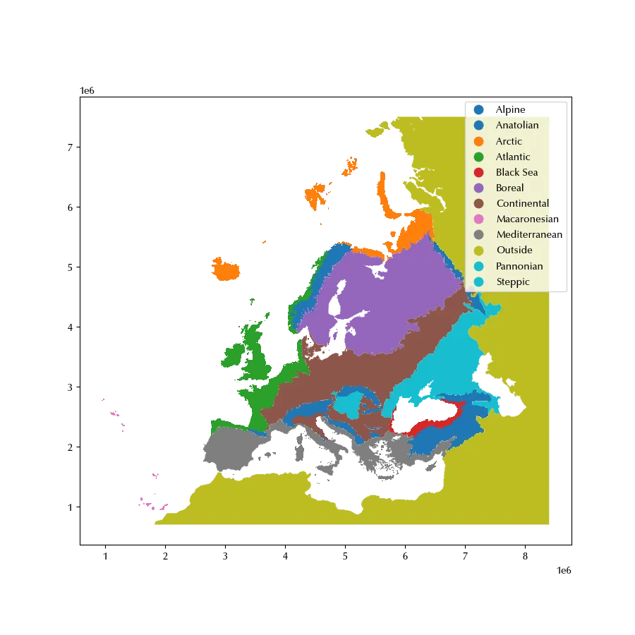
This will be our starting point. First of all, we will drop the ‘Outside’ entry, and we will bring it to a more useful reference frame.
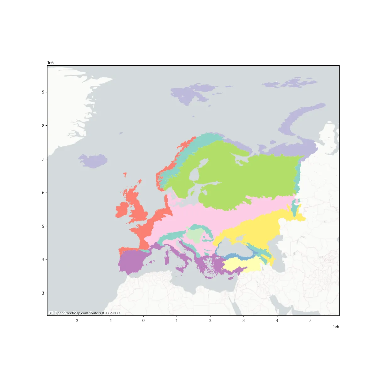
Let us assume we want to compare the size of each biogeographical region, in this case it could be appropriate to use an equal area projection. We will therefore use a Gall-Peters projection. We will also add a basemap, and we will use a minimal one in order to reduce the visual noise. We will also use a softer colormap, since the default one is too vivid. Of course, a custom colormap might be better, but this number of classes it can be tricky to find a good one, and sticking to a pre-designed one will save us a lot of work.
gdf_plot = gdf[gdf['biogeographical_region'] !='Outside'].to_crs(
    pyproj.proj.CRS.from_authority('ESRI', code=54016))

fig, ax = plt.subplots(figsize=(12, 12))
gdf_plot.plot('biogeographical_region', ax=ax, cmap='Set3')
cx.add_basemap(source=cx.providers.CartoDB.PositronNoLabels, ax=ax, crs=gdf_plot.crs, zoom=4)
Adding primary elements
We can now start adding the primary elements of a map. According to “GIS Cartography: a guide to effective map design” they are:
- title
- subtitle
- legend
- map
- north arrow
- date
- authorship
- scale bars
- page border
fig, ax = plt.subplots(figsize=(9, 9))
fig.set_facecolor('lightgray')
ax.set_aspect('auto')
gdf_plot.plot('biogeographical_region', ax=ax, cmap='Set3', legend=True, legend_kwds={'loc': 'lower left'})
cx.add_basemap(source=cx.providers.CartoDB.PositronNoLabels, ax=ax, crs=gdf_plot.crs, zoom=4)
ax.set_title('Biogeographical Regions of Europe', fontsize=18)
ax.add_artist(ScaleBar(1))
north_arrow(
    ax, location="lower right", rotation={"crs": gdf_plot.crs, "reference": "center"}, shadow=False,
)
ax.set_xticks([])
ax.set_yticks([])
ax.patch.set_linewidth(100)
ax.patch.set_edgecolor('lightgray')
fig.tight_layout()
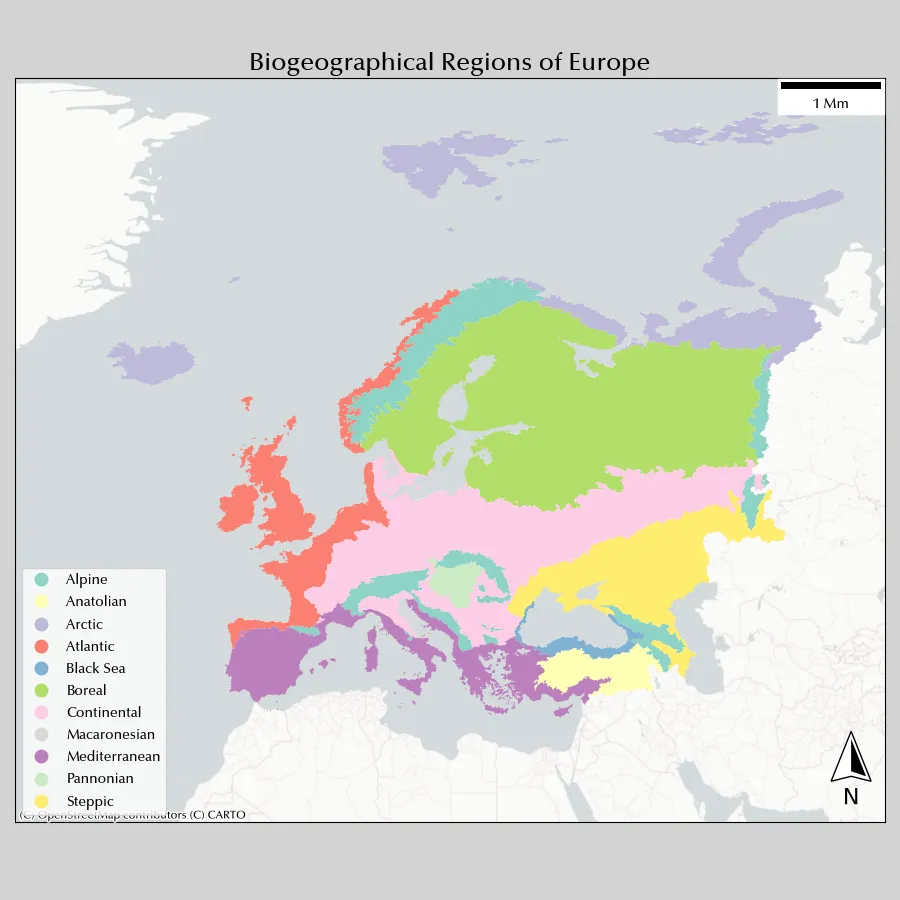
We used the PositronNoLabels map with a zoom equal to 4 since a smaller zoom would not have sufficient to plot our dataset with the required spatial resolution (10 km, which is quite a high resolution for such a large region). The Positron map has another advantage, which is that seas are grey, while other maps has azure seas, and this can create noise with colour categories. Remember that the shown elements depends on the zoom as well as the basemap resolution, so you should always balance the spatial resolution of all of your elements, otherwise the result might be unclear as well as visually unappealing.
We also removed the ticks, since they don’t add any relevant information. We will instead use a graticule, which shows the latitude-longitude grid.
Always remember that matplotlib ticks or grid do not correspond to graticule, since the graticule might be deformed by the projection.
Projected coordinates are not meaningful to most readers, so you should rather project a latitude-longitude graticule.
We downloaded the 15 degrees graticule from the Natural Earth website and used it. We will now add them together with the corresponding annotation for each parallel and meridian.
I am not aware of any fast way to do so in Python (in QGIS this is a one-click operation), so we will take the long way.
gdf_graticule = gpd.read_file('/home/stippe/Downloads/graticule/ne_50m_graticules_15.dbf')

xlim = ax.get_xlim()
ylim = ax.get_ylim()

bds = gpd.GeoDataFrame(geometry=gpd.points_from_xy([xlim[0]], [ylim[0]]), crs=gdf_plot.crs)

xtv = np.arange(-30, 75, 15)
xtl = ['30W', '15W', '0E', '15E', '30E', '45E', '60E']
xtk = gpd.GeoDataFrame(geometry=gpd.points_from_xy(xtv, 0*xtv+bds.to_crs(4326).geometry.y.values[0]), crs=4326
                       ).to_crs(gdf_plot.crs)

ytv = np.arange(30, 90, 15)
ytl = ['30N', '45N', '60N', '75N']
ytk = gpd.GeoDataFrame(geometry=gpd.points_from_xy(0*ytv+bds.to_crs(4326).geometry.x.values[0], ytv), crs=4326
                       ).to_crs(gdf_plot.crs)


fig, ax = plt.subplots(figsize=(9, 8))
fig.set_facecolor('lightgray')
ax.set_aspect('auto')
gdf_plot.plot('biogeographical_region', ax=ax, cmap='Set3', legend=True, legend_kwds={'loc': 'lower left', 'framealpha': 0.4})
cx.add_basemap(source=cx.providers.OpenStreetMap.Mapnik, ax=ax, crs=gdf_plot.crs, zoom=2)
ax.set_title('Biogeographical Regions of Europe', fontsize=18)
# ax.add_artist(ScaleBar(1))
scale_bar(ax, location="upper left", style="boxes", bar={"projection": gdf_plot.crs, "minor_type":"none", 'minor_div': 0, 'major_div': 2, 'max': 2000},
         labels={"loc": "above", "style": "first_last"})
north_arrow(
    ax, location="lower right", rotation={"crs": gdf_plot.crs, "reference": "center"}, shadow=False, scale=0.4
)
gdf_graticule.to_crs(gdf_plot.crs).plot(ax=ax, color='lightgray', lw=0.8)
ax.set_xticks([])
ax.set_yticks([])
xlim = ax.get_xlim()
ylim = ax.get_ylim()
ax.patch.set_linewidth(100)
ax.patch.set_edgecolor('lightgray')
ax.set_xticks(xtk.geometry.x)
ax.set_xticklabels(xtl)
ax.set_yticks(ytk.geometry.y)
ax.set_yticklabels(ytl)
ax.annotate('Date: 2025/05/01', xy=(0, -30), xycoords='axes points', annotation_clip=False)
ax.annotate('Author: S. M.', xy=(0, -45), xycoords='axes points', annotation_clip=False)
ax.annotate('Gall Stereographic projetion', xy=(420, -30), xycoords='axes points', annotation_clip=False)
ax.annotate('Data from Cervellini et al. Biodiversity Data Journal 8', xy=(310, -45), xycoords='axes points', annotation_clip=False)
fig.tight_layout()
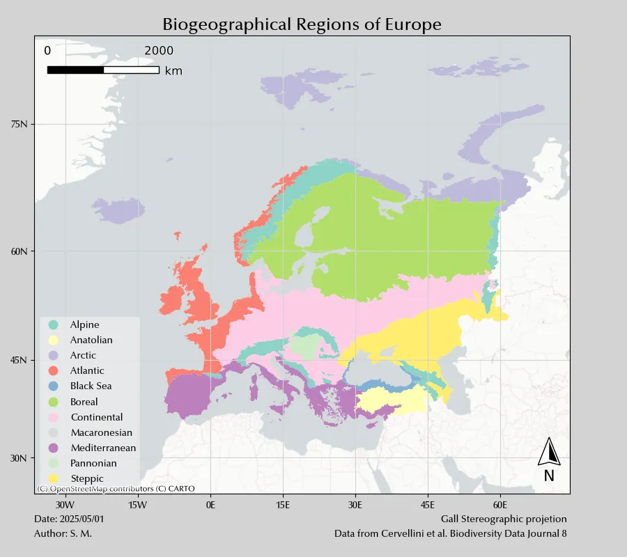
In the last map, we added projection, date and data source, together with the authorship.
We also switched to the scale_bar function, which is more customizable
than the one previously used.
Conclusions
We gave an idea of how to use geopandas to design maps. This is of course only an overview, as there are entire books on this topic.
Suggested readings
- Peterson, G. N. (2009). GIS Cartography: A Guide to Effective Map Design. US: CRC Press.