

Operations on raster data
If you need to manipulate raster data, there are many choices in Python. Which one you prefer using is a matter of taste, and my personal choice is to stick to the xarray ecosystem whenever possible. I do so because I am used to xarray, since PyMC heavily relies on it, and since I am a lazy person, I prefer re-using my knowledge rather than learning a new framework, unless I need to do so. Here we will see how to use the libraries belonging to this ecosystem to manipulate geo-referenced raster data. The libraries we will use are
- xarray as low level library to manipulate raster data
- rasterio to read/write raster files
- rioxarray to let the above libraries talk
- xarray-spatial to simplify operations such as computing zonal statistics or convolutions Of course, we will also use the “usual” libraries such as geopandas, numpy, matplotlib etc.
A little bit more about raster data
In our previous post on raster data we said that, in each raster pixel, there is a stored value. This is however a little oversimplification, since raster files are made by layers, and each layer is a matrix. As an example, jpeg images are made by three layers, where each layer contains integer numbers ranging rom 0 to 255. We usually use tiff files, and they can be made by an arbitrary number of layers. As an example, satellite images can be made by more than 3 layers, and each layer corresponds to a particular sensor in the satellite. Let us see this with an example
from rasterio.plot import show, show_hist, adjust_band
import rasterio
# from rasterio.mask import mask
from rasterio import features
# from rasterio.windows import from_bounds
# from rasterio.transform import Affine
import rioxarray as rxr
import xarray as xr
from xrspatial import convolution, zonal_stats
import xrspatial as xrs
import numpy as np
import pandas as pd
import geopandas as gpd
from matplotlib import pyplot as plt
from pprint import pprint


url = 'https://github.com/thestippe/thestippe.github.io/raw/refs/heads/main/docs/assets/images/turin_bands_all_v2.tiff'
rxarr = rxr.open_rasterio(url)

rxarr.attrs
'AREA_OR_POINT': 'Area',
'_FillValue': np.int16(-32768),
'scale_factor': 1.0,
'add_offset': 0.0,
'long_name': ('B02', 'B03', 'B04', 'B08')}
The last like tells us that there are four different layers. Since they have been downloaded using OpenEO, and in particular they are Landsat 2 images, they correspond to blue, green, red and near-infrared bands. We will see in a future post how to download them using OpenEO. Let us visualize the data in the visible band. Remember that this is simply a reconstruction of the data, obtained by averaging many images obtained over months.
true_col = xrs.multispectral.true_color(rxarr.sel(band=3), rxarr.sel(band=2), rxarr.sel(band=1))
fig, ax = plt.subplots()
true_col.plot.imshow(ax=ax)
fig.tight_layout()
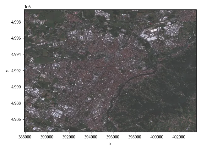
The above images shows the city of Turin, in the north of Italy, and the river in the picture is the Po river, the largest italian river.
In the above code snippet, we reordered the bands as R, G and finally B. Let us see which is the crs of the above image.
print(rxarr.rio.crs)
The NDVI index
We will now calculate the Normalized Difference Vegetation Index (NDVI), which can be calculated as
\[X_{NDVI} = \frac{X_{NIR}-X_R}{X_{NIR}+X_R}\]where $X_{NIR}$ is the scaled near-infrared value, $X_R$ is the scaled red value.
ndvi = xrs.multispectral.ndvi(rxarr.sel(band=4), rxarr.sel(band=3))

fig, ax = plt.subplots()
show(ndvi,
    transform=rxarr.rio.transform(), ax=ax)
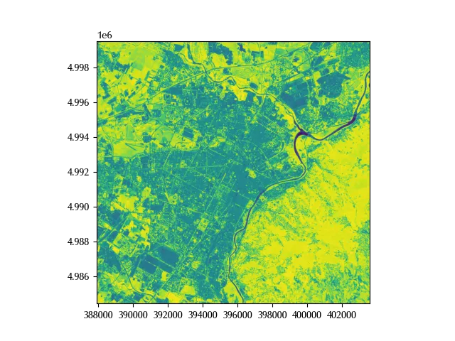
Yellow zones have a higher NDVI than darker zones, so the area with more vegetation is the one on the east of the river.
Clipping the raster data
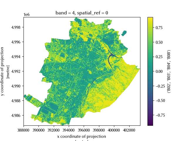
When you work with raster files, you will rarely start your project with files covering exactly the area you are analyzing, so you will generally have to clip them. This can be easily done if you have a geodataframe, a geometry or some shapefile.
gdf = gpd.read_file('ex_quartieri.dbf')
clipped = ndvi.rio.clip(gdf.to_crs(rxarr.rio.crs)['geometry'])
clipped=clipped.where(clipped>-2, np.nan)
fig, ax = plt.subplots()
clipped.plot(ax=ax, cmap='viridis')
Other spatial operations
There are many kinds of operations which can be performed on raster data, and a common operation classification scheme among GIS people is the following one:
- local operations,
- focal operations,
- zonal operations,
- global operations.
We will now give a demonstration of how these kinds of operations can be easily implemented in Python
Local operations
Local operations are those operations where the result at a given raster point only depends on the value at the same point. Local operations can be further classified in unary operations, such as $x \rightarrow 2\times x$, or binary operations, such as $x, y \rightarrow x+y$. The NIR index formula is an example of this kind of operation.
Focal operations
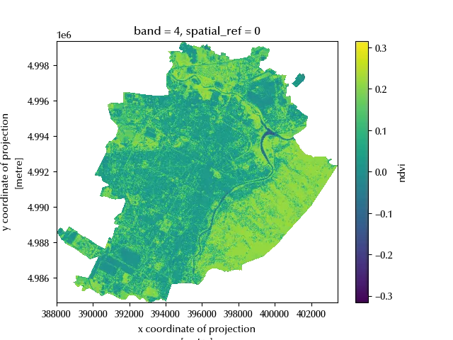
Foca operations are essentially convolutions performed by means of some kernel. These could be, in principle, performed by using xarray or numpy, but using xarray-spatial makes these operations much simpler.
In our example, we will use a blurring kernel to average the NDVI value over the (queen) nearest neighbors (NN). We recall that the rook NN are those on the same row or column, while the queen ones also include the diagonal ones.
filtered = ndvi.copy()
kernel = np.array([[1,2,1],[2,8,2], [1,2,1]])/16

filtered_values = convolution.convolve_2d(ndvi.values, kernel)

filtered.values = filtered_values

fig, ax = plt.subplots()
(filtered-ndvi).rio.clip(gdf.to_crs(rxarr.rio.crs)['geometry']).plot(ax=ax, cmap='viridis')
Zonal operations
In order to perform zonal operations, we need two raster objects:
- in one object we store the variable of interest, e.g. the NDVI
- in the second one the values are the zones where we want to summarize the variable of interest
Zones can be defined in many possible ways, as an example by means of a local categorization of some variable (e.g. we stratify by altitude). In many cases, however, we need to do so by starting from polygonal vector objects.
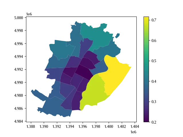
In the following example, we will use Turin’s boros to define the zones,
stored in the IDQUART variable
fields = gdf[['geometry', 'IDQUART']].to_crs(rxarr.rio.crs).values.tolist()

fields_rasterized = features.rasterize(fields, out_shape=ndvi.shape, transform=ndvi.rio.transform())

fields_rasterized_xarr = ndvi.copy()
fields_rasterized_xarr.data = fields_rasterized

df_zonal_stats = zonal_stats(fields_rasterized_xarr, ndvi)

df_zonal_stats.head()
| zone | mean | max | min | sum | std | var | count | |
|---|---|---|---|---|---|---|---|---|
| 0 | 0 | 0.5615 | 0.926978 | -0.534766 | 595231 | 0.283002 | 0.0800903 | 1.06007e+06 |
| 1 | 1 | 0.199839 | 0.873954 | -0.413408 | 7633.46 | 0.196912 | 0.0387744 | 38198 |
| 2 | 2 | 0.241116 | 0.877341 | -0.373802 | 5902.77 | 0.232254 | 0.0539419 | 24481 |
| 3 | 3 | 0.255152 | 0.834259 | -0.118406 | 7090.67 | 0.19375 | 0.0375389 | 27790 |
| 4 | 4 | 0.245008 | 0.848548 | -0.0598135 | 5417.61 | 0.202779 | 0.0411193 | 22112 |
In the above table, the zone 0 corresponds to the region outside from
the city perimeter, while the remaining zones correspond to the IDQUART variable.
gdf_stats = gdf.merge(df_zonal_stats, left_on='IDQUART', right_on='zone')
fig, ax = plt.subplots()
gdf_stats.plot('mean', ax=ax, legend=True)
Global operations
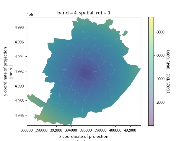
If the result of an operation at one point depends on the value of all the input raster points, such operation is said to be a global operation. A typical example of global operation is the distance from one point. As usual, this can be easily calculated with xarray.
# We first compute the centroid of Turin

warr.values = np.invert(np.isnan(clipped.values)).astype(int)
xc = warr.x.weighted(warr.fillna(0)).mean().values
yc = warr.y.weighted(warr.fillna(0)).mean().values

## We now compute the distance of each point in turin from the centroid
dist_mat = ndvi.copy()

xv = np.array(ndvi.x)-xc
yv = np.array(ndvi.y)-yc

xa, ya = np.meshgrid(xv, yv)

dist_mat.values = np.sqrt(xa**2 + ya**2)
dist_mat = dist_mat.rio.clip(gdf.to_crs(dist_mat.rio.crs)['geometry'])
dist_mat=dist_mat.where(dist_mat>0, np.nan)

# We finally plot the result

fig, ax = plt.subplots()
gdf.to_crs(dist_mat.rio.crs).plot(ax=ax)
dist_mat.plot(ax=ax, cmap='viridis', alpha=0.4)
Conclusions
With the xarray ecosystem you can easily manipulate raster data and perform any kind of operation you commonly need to perform in GIS.
%load_ext watermark
%watermark -n -u -v -iv -w
Python implementation: CPython
Python version : 3.12.8
IPython version : 8.31.0
rasterio : 1.4.3
rioxarray : 0.18.2
matplotlib: 3.10.1
numpy : 2.1.3
xrspatial : 0.4.0
pandas : 2.2.3
xarray : 2025.1.1
geopandas : 1.0.1
Watermark: 2.5.0