

Operations on vector data
One of the first things you learn as a data scientist is how to process tabular data. Either by using pandas or by using some SQL language, you learn how to filter, transform, group or combine data.
The same kind of concepts can be applied to spatial data, and here we will show how to perform some very basic operations.
Geopandas supports all the operations supported by pandas. We won’t discuss the basic pandas operations here, and we will assume that the reader is already familiar with them.
Single layer operations
The simplest kind of operations you can perform with vector data are operations involving one layer at time, that is single layer operations.
Buffering
Buffering implies the creation of a region of given width around a geometry, either points, lines or polygons. Let us consider the municipalities geodataframe, already introduced in this post.
import numpy as np
import pandas as pd
import geopandas as gpd
from matplotlib import pyplot as plt

gdf_comuni = gpd.read_file('/home/stippe/Downloads/comuni_piemonte/Ambiti_Amministrativi-Comuni.shp')

gdf_regione = gdf_comuni.dissolve()

fig, ax = plt.subplots()
gdf_regione.buffer(10000).plot(ax=ax, color='gray')
gdf_regione.plot(ax=ax, color='lightgray')
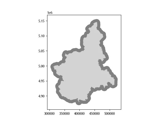
In the above snippet we first performed the dissolve operation, which we will
soon discuss, and then we plotted the dissolved polygon, in light gray, together with the same
polygon with a buffer of 10000 meters, which is shown in darker gray.
Dissolve and explode
We already used the dissolve method in its simplest form, which simply
groups all the geometries into a single geometry.
This method can also be used by selecting one or more grouping columns,
and it is analogous to the groupby SQL or pandas method.
You can also specify an aggregating function, as you would do with the groupby.
gdf_prov = gdf_comuni.dissolve(by='provin_nom').reset_index()
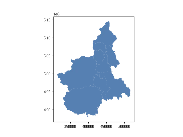
The action of splitting a composite geometry as multipolygons into simple geometries
as polygons can be performed by using the explode method.
gdf_prov[gdf_prov['provin_nom']=='CUNEO']['geometry']
gdf_prov[gdf_prov['provin_nom']=='CUNEO']['provin_nom'].value_counts()
CUNEO 1
Name: count, dtype: int64
gdf_prov_exploded = gdf_prov.explode().reset_index()
gdf_prov_exploded[gdf_prov_exploded['provin_nom']=='CUNEO']['provin_nom'].value_counts()
CUNEO 2
Name: count, dtype: int64
As you can see, while “CUNEO” was only present in one row in the initial geodataframe, it was present into two rows in the exploded one. We can also inspect the geeometry type of the corresponding rows.
type(gdf_prov[gdf_prov['provin_nom']=='CUNEO']['geometry'].values[0])
type(gdf_prov_exploded[gdf_prov_exploded['provin_nom']=='CUNEO']['geometry'].values[1])
Multiple layer operations
Operations involving two oe more layer are also known as multiple layer operations, and here we will give an overview of the most common ones. Always keep in mind that all the geodataframe must be expressed into the same CRS.
Clip
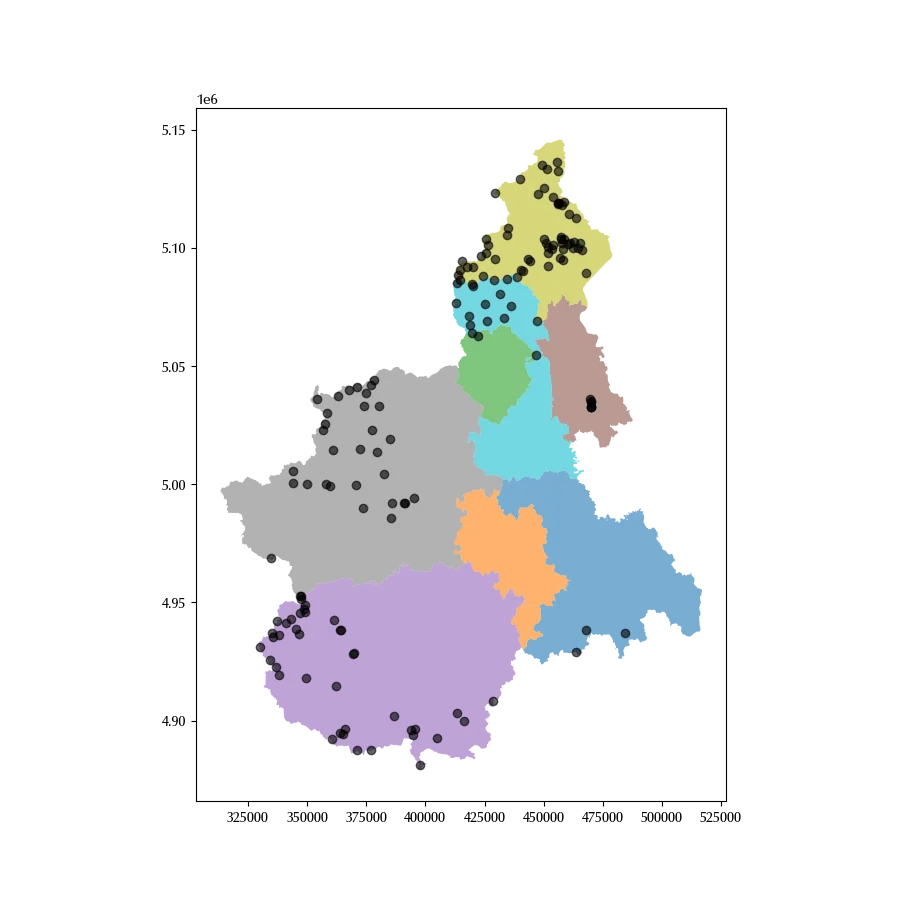
Clipping is the operation to restrict one geodataframe to the area covered by a (polygonal) clipping geodataframe. It also happens that one layer covers an area wider than needed, so clipping is a quite frequent operation. We already introduced the mountain refuges dataset in a previous post, and we recall that it included list of the mountain refuges in Italy. Let us assume that we want to restrict to a specific italian region, namely Piedmont. We can do this as follows
fig, ax = plt.subplots(figsize=(9, 9))
gdf_prov.plot('provin_nom', alpha=0.6, ax=ax)
gdf_rifugi.clip(gdf_prov).plot(ax=ax, color='k', alpha=0.6)
Overlay
Overlay operations are boolean operations as union, intersection or set difference
between geometries, and they can be performed with the overlay
method.
fig, ax = plt.subplots()
gdf_regione.boundary.plot(ax=ax, color='k')
gdf_parchi.plot(ax=ax, color='C1')
gdf_regione.overlay(gdf_parchi, how='intersection').plot(ax=ax)
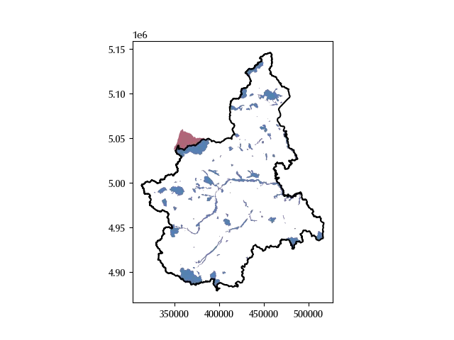
In the above figure, the red region is the one excluded by the overlay operation, as the corresponding park belongs to two different italian regions.
Spatial join
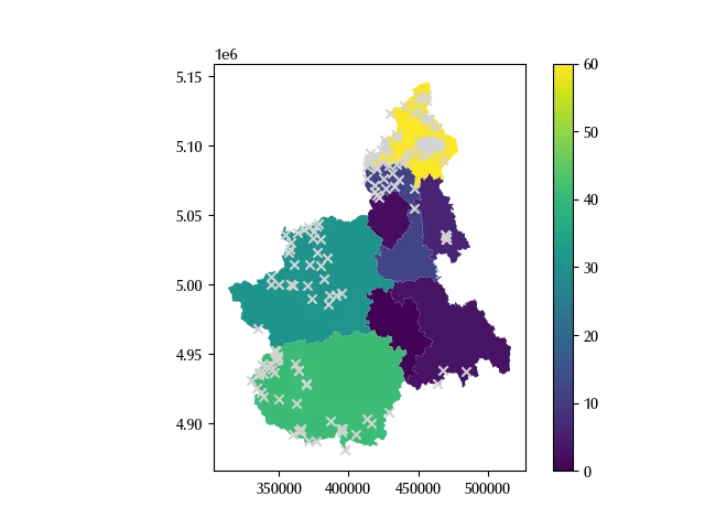
A spatial join is a join which inherits the geometry of the left hand geodataframe, but uses a spatial boolean operation as predicate. Let us assume we want to count the number of refuges for each province, we can do this as follows:
- we first perform a spatial join between the province geodataframe and the refuges one
- we then dissolve by province
- we aggregate by using the count function
gdf_rifugi_piemonte = gdf_rifugi.to_crs(gdf_regione.crs).clip(gdf_regione)

gdf_rifugi_per_provincia = gdf_prov.sjoin(gdf_rifugi_piemonte, how='left').dissolve(by="provin_nom",
     aggfunc={

         "Longitudine": "count",

     })

fig, ax = plt.subplots()
gdf_rifugi_per_provincia.reset_index().plot('Longitudine', legend=True, ax=ax)
gdf_rifugi.clip(gdf_regione).plot(ax=ax, marker='x', color='lightgray')
Sjoin nearest
The sjoin_nearest method is a join which can be used into two ways
- by default, it joins each unit of the left geodataframe with the nearest unit of the right one
- if a distance is specified, then it joins each unit of the left gdf with all the units of the right one within the given distance.
The resulting geometry is always the one of the left gdf.
Let us first clean a little bit our gdfs
gdf_sentieri_principali = gdf_sentieri[(np.invert(gdf_sentieri['DESCRIZION'].isnull()))].dissolve(
    by='DESCRIZION').reset_index()
gdf_filt = gdf_prov[gdf_prov['provin_nom']=='VERBANO-CUSIO-OSSOLA']

gdf_rifugi_vc = gdf_rifugi_piemonte.clip(gdf_filt)
gdf_sentieri_vc = gdf_sentieri_principali.clip(gdf_filt)
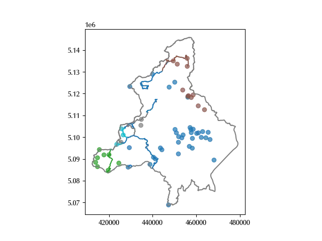
We can now perform the sjoin nearest and associate each mountain refuge to the nearest hiking route
gdf_rifugi_per_sentiero = gdf_rifugi_vc.sjoin_nearest(gdf_sentieri_vc, how='inner')

gdf_rifugi_per_sentiero.sort_values(by='DESCRIZION', inplace=True)

gdf_sentieri_vc.sort_values(by='DESCRIZION', inplace=True)

gdf_sentieri_filt = gdf_sentieri_vc[gdf_sentieri_vc['DESCRIZION'].isin(
    gdf_rifugi_per_sentiero['DESCRIZION'])]

fig, ax = plt.subplots()
gdf_filt.boundary.plot(ax=ax ,color='gray')
gdf_sentieri_filt.sort_values(by='DESCRIZION').plot('DESCRIZION', ax=ax)
gdf_rifugi_per_sentiero.sort_values(by='DESCRIZION').plot('DESCRIZION', ax=ax, alpha=0.7)
Conclusions
We introduced the main categories of vector data operations, and we have seen how to implement them by using GeoPandas.
%load_ext watermark
%watermark -n -u -v -iv -w
Python implementation: CPython
Python version : 3.12.8
IPython version : 8.31.0
matplotlib: 3.10.1
numpy : 2.2.5
shapely : 2.1.0
geopandas : 1.0.1
pandas : 2.2.3
Watermark: 2.5.0