

101 ways to reproject your data
In an old post we discussed how to choose a projection. In this post we will get our hands a little bit more dirty, and we will show some of the most common ways to select the crs. We will PyPROJ, which is a Python wrapper for PROJ.
As datasets, we will the Biology of birds practical, which is a small dataset describing the GPS track of some bird, made available by Luke Ozsanlav-Harris for teaching purposes.
import geopandas as gpd
from matplotlib import pyplot as plt
from pyproj import CRS
from pyproj.aoi import AreaOfInterest
from pyproj.database import query_utm_crs_info, get_authorities

gdf = gpd.read_file('birds/points.shp')
bounds = gpd.read_file('https://raw.githubusercontent.com/martynafford/natural-earth-geojson/refs/heads/master/50m/physical/ne_50m_coastline.json')

bounds.crs
Name: WGS 84
Axis Info [ellipsoidal]:
- Lat[north]: Geodetic latitude (degree)
- Lon[east]: Geodetic longitude (degree)
Area of Use:
- name: World.
- bounds: (-180.0, -90.0, 180.0, 90.0)
Datum: World Geodetic System 1984 ensemble
- Ellipsoid: WGS 84
- Prime Meridian: Greenwich
gdf.crs==bounds.crs
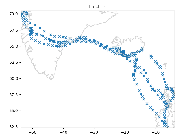
The two datasets are encoded with the same CRS, which is the latitude-longitude one. Let us first of all take a look at the raw data.
crs = gdf.crs
minx, miny = tuple(gdf.to_crs(crs).bounds[["minx", "miny"]].min().values)
maxx, maxy = tuple(gdf.to_crs(crs).bounds[["maxx", "maxy"]].max().values)
fig, ax = plt.subplots()
bounds.to_crs(crs).plot(ax=ax, color="lightgray")
gdf.to_crs(crs).plot(ax=ax, marker='x')
ax.set_xlim([minx, maxx])
ax.set_ylim([miny, maxy])
ax.set_title("Lat-Lon")
fig.tight_layout()
In pyproj there are many ways to choose the CRS, and the most common ones
are from_epsg, from_user_input and from_string.
These functions are really easy to use,
and from_epsg(XXXX) is equivalent to from_user_input(XXXX)
and to from_string("ESPG:XXXX"").
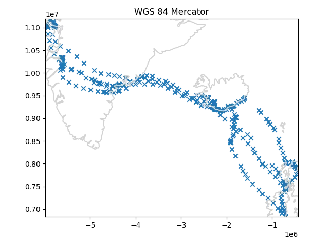
crs = CRS.from_epsg(3395)
# equivalent: CRS.from_user_input(3395) or CRS.from_string("EPSG:3395")
minx, miny = tuple(gdf.to_crs(crs).bounds[["minx", "miny"]].min().values)
maxx, maxy = tuple(gdf.to_crs(crs).bounds[["maxx", "maxy"]].max().values)
fig, ax = plt.subplots()
bounds.to_crs(crs).plot(ax=ax, color="lightgray")
gdf.to_crs(crs).plot(ax=ax, marker='x')
ax.set_xlim([minx, maxx])
ax.set_ylim([miny, maxy])
ax.set_title("WGS 84 Mercator")
fig.tight_layout()
Each area has its own typical projections, so if you are used to map a certain area, you will likely be familiar with the EPSG codes of these projections. As an example, I know by heart that the 3003/3004 projection are the Monte Mario projections, while EPSG: 32632 to EPSG: 32634 are UTM WGS 84 32N-34N, and these are typical projections used in Italy.
In particular, UTM projections are very common when you must work on the country level. If you are working on a map of some country you are not familiar with, you might want to find the associated UTM projections.
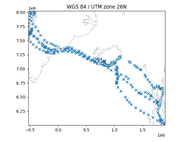
Pyproj allows you to easily find the UTM projections associated with a given area, and you can do this as follows.
crs = bounds.crs
minx, miny = tuple(gdf.to_crs(crs).bounds[["minx", "miny"]].min().values)
maxx, maxy = tuple(gdf.to_crs(crs).bounds[["maxx", "maxy"]].max().values)
utm_crs_list = query_utm_crs_info(
    datum_name="WGS 84",
    area_of_interest=AreaOfInterest(
        west_lon_degree=minx,
        south_lat_degree=miny,
        east_lon_degree=maxx,
        north_lat_degree=maxy,
    ),
)

utm_crs = CRS.from_epsg(utm_crs_list[len(utm_crs_list)//2].code)

crs = utm_crs
minx, miny = tuple(gdf.to_crs(crs).bounds[["minx", "miny"]].min().values)
maxx, maxy = tuple(gdf.to_crs(crs).bounds[["maxx", "maxy"]].max().values)
fig, ax = plt.subplots()
bounds.to_crs(crs).plot(ax=ax, color="lightgray")
gdf.to_crs(crs).plot(ax=ax, marker='x')
ax.set_xlim([minx, maxx])
ax.set_ylim([miny, maxy])
ax.set_title(f"{utm_crs.name}")
fig.tight_layout()
Not all projections have an associated EPSG code, so you might
be interested in using a projection which is encoded by some authority
which is not EPSG.
You can do this by using the from_authority function.
The list of the available authorities can be obtained as
get_authorities()
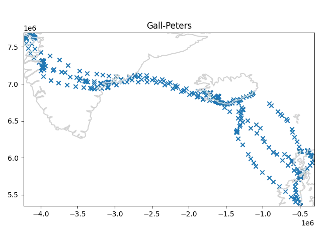
As an example, the Gall-Peters projection has an ESRI code, but it has no EPSG code.
crs = CRS.from_authority('ESRI', code=54016)
minx, miny = tuple(gdf.to_crs(crs).bounds[["minx", "miny"]].min().values)
maxx, maxy = tuple(gdf.to_crs(crs).bounds[["maxx", "maxy"]].max().values)
fig, ax = plt.subplots()
bounds.to_crs(crs).plot(ax=ax, color="lightgray")
gdf.to_crs(crs).plot(ax=ax, marker='x')
ax.set_xlim([minx, maxx])
ax.set_ylim([miny, maxy])
ax.set_title("Gall-Peters")
fig.tight_layout()
In some situation, you might be interested in a deeper customization, because you want to preserve some particular property in your analysis.
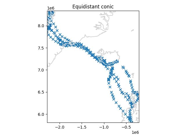
In these cases, simply using a code might not be enough, and you might look for choosing the exact tangent point of your map. In this case you can use the proj syntax. In our case, we will use the equidistant conic projection with latitude equal to the median of the latitude of our GPS points.
crs = CRS.from_proj4(f"+proj=eqdc +lat_1={gdf.geometry.y.median()}")
minx, miny = tuple(gdf.to_crs(crs).bounds[["minx", "miny"]].min().values)
maxx, maxy = tuple(gdf.to_crs(crs).bounds[["maxx", "maxy"]].max().values)
fig, ax = plt.subplots()
bounds.to_crs(crs).plot(ax=ax, color="lightgray")
gdf.to_crs(crs).plot(ax=ax, marker='x')
ax.set_xlim([minx, maxx])
ax.set_ylim([miny, maxy])
ax.set_title("Equidistant conic")
fig.tight_layout()
Conclusions
We have seen how to choose our own projection with pyproj, starting from the simpler methods up to the powerful proj syntax.
%load_ext watermark
%watermark -n -u -v -iv -w
Python implementation: CPython
Python version : 3.12.8
IPython version : 8.31.0
matplotlib: 3.10.1
geopandas : 1.0.1
pyproj : 3.7.1
Watermark: 2.5.0