

Raster data
In this post, we are going to introduce the remaining most common data format you will encounter in GIS, namely raster data. As we previously explained, raster data corresponds to tables where, in each entry (pixel), there is a stored value. You are probably already familiar with some common raster file format such as jpeg, png or gif. There are very common formats for ordinary images, but they might not be appropriate for raster data in GIS. In GIS, in fact, it is quite common to work with very high resolution files, and in this case the most common file format is tiff. Let us see how use python to manipulate raster files.
First of all, download the tiff file from this repo. We can then read it and plot it by using rasterio.
import rasterio
import rioxarray
import geopandas as gpd
from rasterio.enums import Resampling
import rasterio.plot
import matplotlib as mpl
import numpy as np
from matplotlib import pyplot as plt
import pandas as pd

img_snow = rasterio.open('./data/OSMap_Grayscale.tif')

fig = plt.figure()
ax = fig.add_subplot(111)
rasterio.plot.show(img_snow.read(1), cmap='grey', transform=img_snow.transform, ax=ax)
fig.tight_layout()
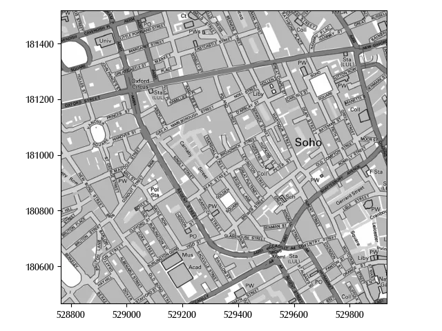
Notice that we used read(1) since there might be more than one band, and the band number starts from 1.
Rasterio is a very popular library, and it does a great job if you are not working with huge files. Unfortunately, when working with spatial data, you will often need to manipulate very large files. This is however not an issue, as there are great high-performance tools for this. The first one is xarray, and we already extensively used it in the statistics section of the blog. There is a separate library, named rioxarray, which allows you to load raster data as xarray objects.
Let us try it with an example. We downloaded the tiff file (as well as the sld file) which you can find at this link from the ISPRA website.
xds = rioxarray.open_rasterio('./data/Copertura_del_suolo_2023.tif')
xds.shape
The tiff file has a size of almost 600 MB, and it consists of roughly $10^5 \times 10^5 = 10^{10}$ pixels. Unless you have tons of RAM, I would not recommend you to naively manipulate it as a numpy array, or your PC could easily crash. However, by using xarray and being a little smart, you can comfortably handle it.
Let us continue with our example of the Piedmont region.
gdf_municipalities = gpd.read_file('./data/municipalities/Ambiti_Amministrativi-Comuni.dbf')
We will first clip it by manually, as this requires less memory than it requires doing it by using xarray.
geom=gdf_municipalities.to_crs(xds.spatial_ref.crs_wkt).dissolve()
geom.bounds
| minx | miny | maxx | maxy | |
|---|---|---|---|---|
| 0 | 4.05517e+06 | 2.33056e+06 | 4.25866e+06 | 2.59582e+06 |
Notice that we projected the vector data on the crs of the raster data, as doing the opposite introduces approximation errors.
Now that our dataset has a manageable size, let us take a closer look at its content
np.unique(xds_red.values)
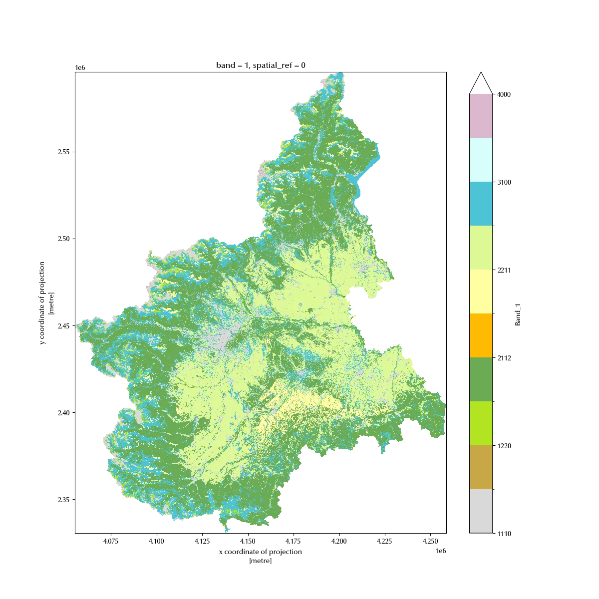
There are 12 different values, each corresponding to a different soil type (which is encoded into the other file we downloaded). Raster data can contain any kind of datum, float, integer ( which may corresponds to count), bool…
We can now clip our xarray as we would do with a dataframe
filtx =(xds.x.values>=geom.bounds.minx.iloc[0]) & (xds.x.values<=geom.bounds.maxx.iloc[0])
filty =(xds.y.values>=geom.bounds.miny.iloc[0]) & (xds.y.values<=geom.bounds.maxy.iloc[0])
xds_red = xds[0, filty, filtx]
xds_red.shape
This size is a little bit better, but we can further reduce the size of our file, since we still have a matrix containing roughly $10^9$ entries. The original dataset has a spatial resolution of $10m \times 10m$, which is far too high for our purposes. We can safely downsample it to a resolution of $50m \times 50m$ as follows
downscale_factor = 4
new_width = int(xds_red.rio.width / downscale_factor)
new_height = int(xds_red.rio.height / downscale_factor)

xds_downsampled = xds_red.rio.reproject(
    xds_red.rio.crs,
    shape=(new_height, new_width),
    resampling=Resampling.mode,
)

xds_downsampled.shape
We are only interested in the Piedmont region, and we can now clip the xarray to the geodataframe.
clipped = xds_downsampled.rio.clip(geom.geometry, geom.crs)
Before plotting the result, let us now construct the colormap by using the information stored inside the sld file. I constructed a csv file starting from the sld file, with the following entries.
| colour | value | description_ita | description_eng | |
|---|---|---|---|---|
| 0 | #ac2000 | 1110 | Superfici artificiali | Artificial surface |
| 1 | #d9d9d9 | 1210 | Superfici consolidate | Consolidated soil |
| 2 | #c9a846 | 1220 | Superfici non consolidate | Not-consolidated soil |
| 3 | #b3e422 | 2111 | Latifoglie | Broad-leaved trees |
| 4 | #6bab54 | 2112 | Conifere | Conifer trees |
| 5 | #ffbb01 | 2120 | Arbusteti | Shrubby |
| 6 | #ffffa1 | 2211 | Erbaceo periodico | Seasonal grass |
| 7 | #def995 | 2212 | Erbaceo permanente | Perennial grass |
| 8 | #4bc3d5 | 3100 | Corpi idrici | Water bodies |
| 9 | #d7fffb | 3200 | Ghiacciai e nevi perenni | Glaciers |
| 10 | #dbb8cd | 4000 | Zone umide | Wet zones |
cmap, norm = mpl.colors.from_levels_and_colors(df_cmap['value'].values, df_cmap['colour'].values,extend='min')

fig = plt.figure(figsize=(12, 12))
ax = fig.add_subplot(111)
clipped.plot.imshow(cmap=cmap,norm=norm, ax=ax)
Conclusions
Dealing with raster data may seem tricky, but by using the appropriate tools you can efficiently handle even files with billions of pixels and work with high resolution images.
%load_ext watermark
%watermark -n -u -v -iv -w -p xarray
Python implementation: CPython
Python version : 3.12.7
IPython version : 8.24.0
xarray: 2024.9.0
rasterio : 1.3.11
geopandas : 1.0.1
rioxarray : 0.17.0
pandas : 2.2.3
numpy : 1.26.4
matplotlib: 3.9.2
Watermark: 2.4.3