

Vector data
Vector data is one of the most common kind of data you will work with in geographic data analysis. This kind of data is generally obtained by GPS data, but can also be extracted from images or, more generally, from raster data. Here we will introduce vector data, together with some of the simplest and most common operations you can perform with vector data. We will also show how to store, read and visualize vector data.
Reading vector data files with geopandas
Geopandas is one of the most popular tools in Python to handle vector data files. Geopandas can do much more than this, as it allows you to manipulate and visualize vector data. This library is based on Pandas, but it also includes many tools from a variety of different packages and libraries.
One simple way to store point data is to use csv files, where two columns are associated with the coordinates of the point. As an example, we used the dataset in this link to get the list of the mountain refuges in Italy. In this dataset, the columns “Longitudine” and “Latitudine” are associated with the longitude and latitude of each refuge.
import geopandas as gpd
import pandas as pd
import matplotlib as mpl
from matplotlib import pyplot as plt

df = pd.read_csv("./data/Mappa-dei-rifugi-in-Italia.csv", encoding='latin1', sep=';')
gdf = gpd.GeoDataFrame(df, crs='WGS84', geometry=gpd.points_from_xy(df['Longitudine'], df['Latitudine']))
gdf.plot()
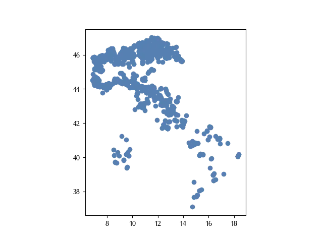
Here we constructed a GeoPandas GeoDataFrame with a Pandas DataFrame. In order to construct a GeoDataFrame we specified the geometry from the columns “Longitudine” and “Latitudine”, and we used the WGS84 (also known as ESPG:4326) coordinate reference system, which is nowadays the most common ellipsoidal crs.
We can also leverage Leaflet to interactively show the above dataset on the OpenStreetMap map as follows:
gdf.explore()
The above method, however, is very limited, as you can only easily store point vector data, and there is no easy way to share the coordinate reference system. For these reasons a more popular way to share vector data is to use shapefiles.
A shapefile consists by a set of files which must stay in the same folder, the most important ones are:
- a shp file, which contains the geometry
- a shx file, containing the index
- a dbf file, containing the attributes
- a (non-mandatory) prj file, containing the projection.
There are other files which may stay inside the same folder and are searched by geopandas or by the GIS file, but they are not mandatory.
We downloaded and unzipped the zip file which can be found at this link to get the list of the municipalities in Piedmont (Italy) into the “municipalities” folder.
gdf_municipalities = gpd.read_file('./data/municipalities/Ambiti_Amministrativi-Comuni.dbf')
gdf_municipalities.plot()
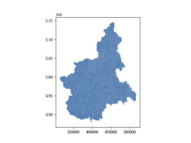
The above is an example of polygon data, while an example of multiline data is the set of hiking/bike routes of Piedmont, which can be downloaded from this link.
gdf_routes = gpd.read_file('.(data/routes/rete_sentieristica.dbf')
gdf_routes.plot()
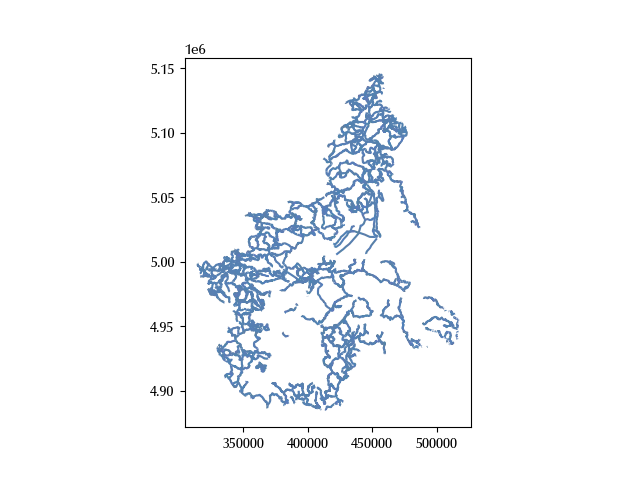
Notice that the coordinates in the refuges dataset are expressed in latitude and longitude, while this is impossible for the other datasets, since the x and y coordinates are order of magnitude larger.
gdf_routes.crs
Name: WGS 84 / UTM zone 32N
Axis Info [cartesian]:
- E[east]: Easting (metre)
- N[north]: Northing (metre)
Area of Use:
- name: Between 6°E and 12°E, northern hemisphere between equator and 84°N, onshore and offshore. Algeria. Austria. Cameroon. Denmark. Equatorial Guinea. France. Gabon. Germany. Italy. Libya. Liechtenstein. Monaco. Netherlands. Niger. Nigeria. Norway. Sao Tome and Principe. Svalbard. Sweden. Switzerland. Tunisia. Vatican City State.
- bounds: (6.0, 0.0, 12.0, 84.0)
Coordinate Operation:
- name: UTM zone 32N
- method: Transverse Mercator
Datum: World Geodetic System 1984 ensemble
- Ellipsoid: WGS 84
- Prime Meridian: Greenwich
gdf_municipalities.crs==gdf_routes.crs
The choice of the crs can affect your calculation and depends on your needs. It is generally better to work with a projected (metric) crs rather than with the unprojected (angular i.e. latitude and longitude) coordinates, we will therefore work with the latter crs. This crs, in particular, is a Universal Transverse Mercator projection, which is a very common kind of projection up to country-level data, but it’s unsuitable for larger (e.g. continent) scale data.
Notice that the refuges dataset contains data for the entire Italy, while the remaining datasets only contain data for the Piedmont region. Since we lack of data for the remaining regions, we will clip the refuge to the Piedmont regions. In other terms, we will construct a sub-dataset which only contains data for the Piedmont region.
We will do this in two steps: first of all, we will construct a polygon shape for the entire Piedmont region, then we will clip the refuges dataset to this region. The first step is necessary since the municipalities dataset contains one polygon for each municipality, and this step can be achieved with the dissolve method
region = gdf_municipalities.dissolve()
We can now clip the refuges dataset to this region, but first we must re-project the refuges dataset to the region crs.
gdf_red = gdf.to_crs(gdf_routes.crs).clip(region)
Another common format to share geodata is by using geojson. We created a small GeoJSON file with the coordinates of the mountains above 4500 meters over the sea level in the “mounts.geojson” file, and the content of this file was the following:
{
  "type": "FeatureCollection",
  "features": [
    {
      "type": "Feature",
      "properties": {
        "name": "Punta Nordend",
	"elevation": 4609
      },
      "geometry": {
        "coordinates": [
          7.850,
          45.933
        ],
        "type": "Point"
      }
    },
    {
      "type": "Feature",
      "properties": {
        "name": "Punta Gnifetti",
	"elevation": 4554
      },
      "geometry": {
        "coordinates": [
           7.877,
          45.927
        ],
        "type": "Point"
      }
    }
  ]
}
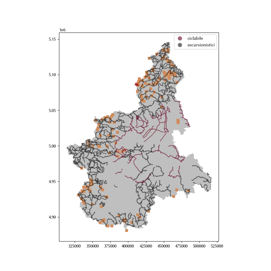
We can finally show the refuges together with the routes and the mountains.
gdf_mounts = gpd.read_file('./data/mounts.geojson')

fig = plt.figure(figsize=(9, 9))
ax = fig.add_subplot(111)
region.plot(ax=ax, color='grey', alpha=0.5)
gdf_routes.plot('TIPOLOGIA', ax=ax, alpha=0.6, legend=True, cmap=mpl.cm.RdGy)
gdf_red.plot(ax=ax, color='#d28b5a', marker='s')
gdf_mounts.to_crs(gdf_routes.crs).plot(ax=ax, color='brown', marker='^')
Conclusions
Vector data is very common in geographic data analysis, and there are plenty of formats to store this kind of data. GeoPandas, however, will simplify your life, by allowing you to read, manipulate and store vector data as you would do with pandas dataframes.
%load_ext watermark
%watermark -n -u -v -iv -w -p folium
Python implementation: CPython
Python version : 3.12.7
IPython version : 8.24.0
folium: 0.17.0
geopandas : 1.0.1
pandas : 2.2.3
matplotlib: 3.9.2
Watermark: 2.4.3