Logistic regression

In the last posts we discussed how to build the simplest regression model for a real variable with the linear model. This model can be used as a starting block to perform regression on many other types of data, and this can be done by building a Generalized Linear Model (GLM).

GLMs can be constructed by starting from any likelihood for the data $P(y | \theta)\,.$

The parameter $\theta$ usually is bounded to some specific range $D$: we have $\theta \in [0, 1]$ for the Binomial likelihood, while we have $\theta > 0$ for the Poisson model. On the other hand, the variable

\[Z \sim \alpha + \beta X\]

can generally take any real value. However, by choosing a suitable function

\[f : \mathbb{R} \rightarrow D\]

we can map our random variable $Z$ to the desired domain $D\,.$

The general GLM can therefore be written as

\[\begin{align} Y & \sim P(\theta) \\ \theta & = f\left(\alpha + \beta X\right) \end{align}\]

Of course $\alpha$ and $\beta$ and any other parameter $\phi$ will be described by a suitable prior distribution.

Let us now see how to do this in practice.

The logistic model

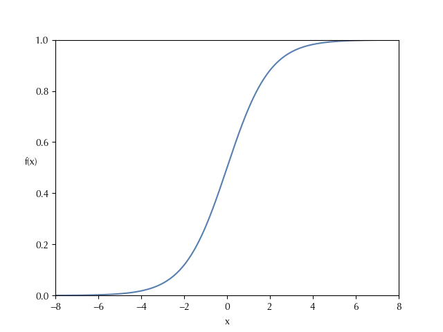
The logistic model can be applied when there is a single binary dependent variable which depends on one or more independent variables, which can be binary, integer or continuous. In the logistic model the likelihood is taken as the binomial one, while the mapping function $f$ is taken as the logistic function, plotted below:

\[f(x) = \frac{1}{1+e^{-x}}\]

The logistic function

We will apply the logistic regression to the Challenger O-ring dataset. On January 28th 1986 the shuttle broke during the launch, killing several people, and the USA president formed a commission to investigate on the causes of the incident. One of the member of the commission was the physicist Richard Feynman, who proved that the incident was caused by a loss of flexibility of the shuttle O-rings caused by the low temperature (see the Wikipedia page) Here we will take the data on the number of O-rings damaged in each mission of the Challenger, and we will provide an estimate on the probability that one o-ring becomes damaged as a function of the temperature. The original data can be found here, and we provide here the dataset grouped by temperature for completeness (the temperature is expressed in °F).

	temperature	damaged	undamaged	count
0	53	5	1	6
1	57	1	5	6
2	58	1	5	6
3	63	1	5	6
4	66	0	6	6
5	67	0	18	18
6	68	0	6	6
7	69	0	6	6
8	70	2	22	24
9	72	0	6	6
10	73	0	6	6
11	75	1	11	12
12	76	0	12	12
13	78	0	6	6
14	79	0	6	6
15	81	0	6	6

The dataset contains all the information collected before the Challenger disaster. The logistic model is already implemented into PyMC, but to see how it works we will implement it from scratch.

import pandas as pd
import pymc as pm
import arviz as az
import numpy as np
from matplotlib import pyplot as plt
import pymc.sampling_jax as pmjax
import seaborn as sns


rng = np.random.default_rng(42)

df_oring= pd.read_csv('./data/orings.csv')

# Convert it to Celsius

df_oring['deg'] = (df_oring['temperature']-32)*5/9

I converted the temperature to Celsius degree because it is easier for me to reason in terms of Celsius degree. Let us write down our model

\[\begin{align} Y_i \sim & \mathcal{Binom}(p_i, n_i)\\ p_i = & \frac{1}{1+e^{-\alpha - \beta X_i}} \\ \end{align}\]

The odds ratio is defined as

\[\begin{align} \frac{p}{1-p} & = \frac{1}{1+e^{-\alpha - \beta X}}\frac{1}{1-\frac{1}{1+e^{-\alpha - \beta X}}} \\ & = \frac{1}{1+e^{-\alpha - \beta X}}\frac{ 1+e^{-\alpha - \beta X} }{e^{-\alpha - \beta X}} \\ & = e^{\alpha + \beta X} \end{align}\]

therefore

\[\log\left(\frac{p}{1-p}\right) = \alpha + \beta X\]

We can therefore identify $\alpha$ with the log odds at $T=0°C$ It doesn’t really make sense to assume either a too big number or a too small one, so we will take

\[\alpha \sim \mathcal{N}(0, 15)\]

On the other hand, $\beta$ represents the variation of the log odds with an increase of $1°C\,.$ We do expect a meaningful variation on a scale of $10°C\,,$ so we can generously take

\[\beta \sim \mathcal{N}(0, 2)\]

We are now ready to implement our model

with pm.Model() as logistic:
    alpha = pm.Normal('alpha', mu=0, sigma=15)
    beta = pm.Normal('beta', mu=0, sigma=2)
    log_theta = alpha + beta*df_oring['deg']
    theta = 1/(1+pm.math.exp(-log_theta))
    y = pm.Binomial('y', p=theta, n=df_oring['count'], observed=df_oring['undamaged'])


with logistic:
    idata_logistic = pm.sample(draws=5000, tune=5000, chains=4,
                               random_seed=rng, nuts_sampler='numpyro')


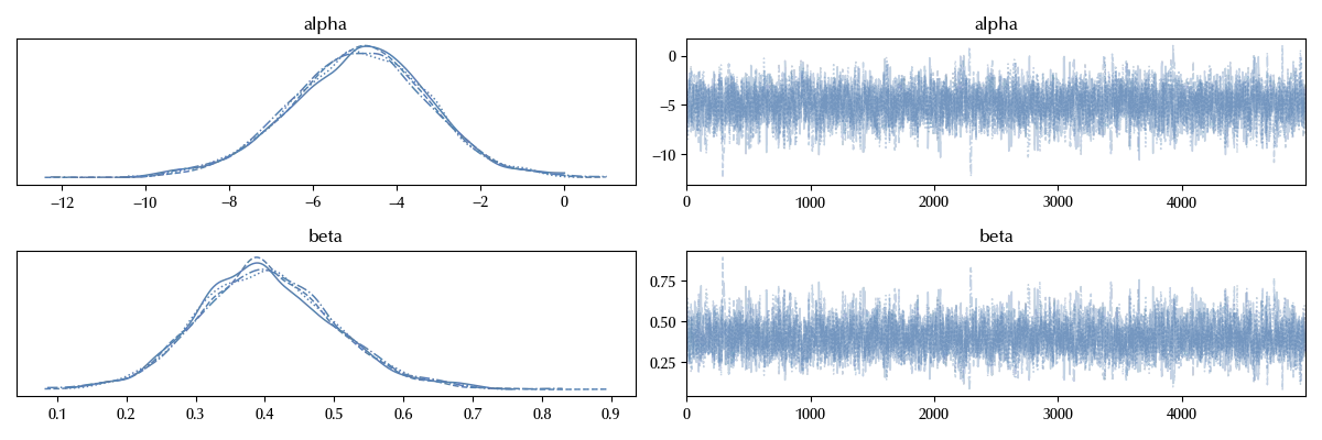
az.plot_trace(idata_logistic)
fig = plt.gcf()
fig.tight_layout()

The trace of the logistic model

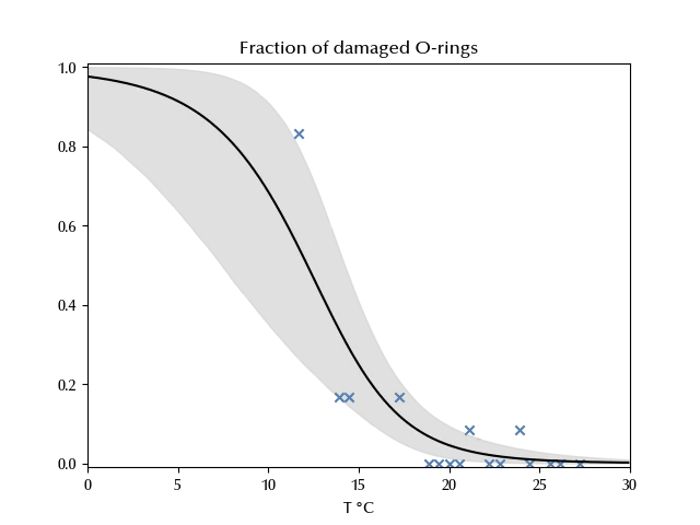
The trace looks fine, we can now take a look at the posterior predictive.

x_pl = np.arange(0, 30, 0.1)

with logistic:
    mu = pm.Deterministic('mu', alpha + beta*x_pl)
    p = pm.Deterministic('p', 1/(1+pm.math.exp(-mu)))

with logistic:
    idata_logistic.extend(pm.sample_posterior_predictive(idata_logistic, var_names=['y', 'mu', 'p'],
                                                        random_seed=rng))

fig = plt.figure()
ax = fig.add_subplot(111)
ax.fill_between(x_pl, 1-
                idata_logistic.posterior_predictive.p.quantile(q=0.025, dim=['draw', 'chain']),
                1-
                idata_logistic.posterior_predictive.p.quantile(q=0.975, dim=['draw', 'chain']),
                color='lightgray', alpha=0.7)

ax.plot(x_pl, 1-
        idata_logistic.posterior_predictive.p.mean(dim=['draw', 'chain']),
        color='k')

ax.scatter(df_oring['deg'], df_oring['damaged']/df_oring['count'],
           marker='x', label='raw data estimate')
ax.set_xlim([0, 30])
ax.set_ylim([-0.01, 1.01])
ax.set_xlabel(r"T $\degree$C")
ax.set_title(r"Fraction of damaged O-rings")

The trace of the logistic model

As we can see, the more we approach $0°\,,$ the more it is likely that an O-ring gets damaged. The forecasted temperature for the launch day was $26-29 °F\,,$ corresponding to a range between $-1.6$ °C and $-3.3$ °C.

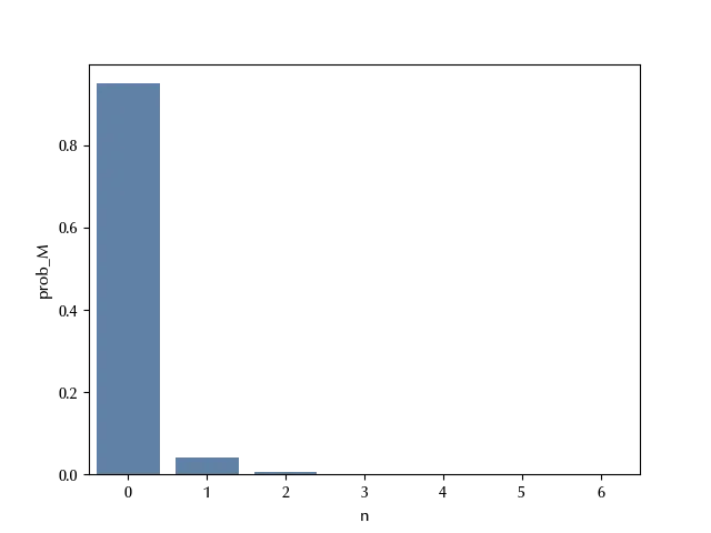
We must however consider that one broken O-ring is not enough to create serious issues. We can therefore estimate the probability as a function of the number of undamaged rings.

tm = (26-32)*5/9
tM = (29-32)*5/9

with logistic:
    theta_m = 1/(1+np.exp(-(alpha + tm*beta)))
    ym = pm.Binomial('ym', p=theta_m, n=6)
    theta_M = 1/(1+np.exp(-(alpha + tm*beta)))
    yM = pm.Binomial('yM', p=theta_M, n=6)

with logistic:
    ppc_t = pm.sample_posterior_predictive(trace_logistic, var_names=['ym', 'yM'])

# We count how many O-rings are undamaged for each draw

hm = [(ppc_t.posterior_predictive['ym'].values.reshape(-1)==k).astype(int).sum() for k in range(7)]
hM = [(ppc_t.posterior_predictive['yM'].values.reshape(-1)==k).astype(int).sum() for k in range(7)]
h_0 = [k for k in range(7)]

# And we now estimate the corresponding probability

df_h = pd.DataFrame({'n': h_0, 'count_m': hm, 'count_M': hM})
df_h['prob_m'] = df_h['count_m']/df_h['count_m'].sum()
df_h['prob_M'] = df_h['count_M']/df_h['count_M'].sum()

df_h = pd.DataFrame({'n': h_0, 'count_m': hm, 'count_M': hM})

# Let us take a look at the best-case scenario
sns.barplot(df_h, x='n', y='prob_M')

The probaility as a function of the undamaged rings

df_h[df_h['n']==0]['prob_M']

0 0.9469
Name: prob_M, dtype: float64

The most probable scenario is that all O-rings get damaged, and this is scenario has, according to our model, the $95\%$ or probability to happen.

We can conclude that, with the available information, it was not safe to perform the launch. This is however a post-hoc analysis (an analysis performed on some data once the outcome is known), and one should be really careful to draw conclusions based on this kind of analysis, as this easily results into false positive errors (see the Wikipedia page on this topic).

Conclusions

We introduced the Generalized Linear Model, and we analyzed the Challenger dataset by means of a logistic regression. We have seen how, by means of the GLM, we can easily extend the linear regression to binary data. In the next post we will discuss the Poisson regression.

	temperature	damaged	undamaged	count
0	53	5	1	6
1	57	1	5	6
2	58	1	5	6
3	63	1	5	6
4	66	0	6	6
5	67	0	18	18
6	68	0	6	6
7	69	0	6	6
8	70	2	22	24
9	72	0	6	6
10	73	0	6	6
11	75	1	11	12
12	76	0	12	12
13	78	0	6	6
14	79	0	6	6
15	81	0	6	6

	temperature	damaged	undamaged	count
0	53	5	1	6
1	57	1	5	6
2	58	1	5	6
3	63	1	5	6
4	66	0	6	6
5	67	0	18	18
6	68	0	6	6
7	69	0	6	6
8	70	2	22	24
9	72	0	6	6
10	73	0	6	6
11	75	1	11	12
12	76	0	12	12
13	78	0	6	6
14	79	0	6	6
15	81	0	6	6

The logistic model

Conclusions

Suggested readings

	temperature	damaged	undamaged	count
0	53	5	1	6
1	57	1	5	6
2	58	1	5	6
3	63	1	5	6
4	66	0	6	6
5	67	0	18	18
6	68	0	6	6
7	69	0	6	6
8	70	2	22	24
9	72	0	6	6
10	73	0	6	6
11	75	1	11	12
12	76	0	12	12
13	78	0	6	6
14	79	0	6	6
15	81	0	6	6