Mixture models

In mixture models, the distribution is taken as a linear combination of simpler distribution:

\[P(Y | \theta, \omega) = \sum_{i} P_i(Y | \theta_i) \omega_i\]

In the above formula

\[0 \leq \omega_i \leq 1\]

and

\[\sum_i \omega_i = 1\]

Therefore, our observation has been generated according to the probability distribution $P_i$ with probability $\omega_i\,.$

Normal mixture model

The normal mixture is a very common model, and it is also used in machine learning for unsupervised classification. It can be a quick and dirty way to make inference on multimodal data i.e. data which shows than one peak. We will use seaborn’s “geyser” dataset to show an implementation of a normal mixture model. In order to simplify our discussion, we will only deal with the “duration” dimension, but the extension to the multivariate normal is straightforward.

import random
import pandas as pd
import scipy
import numpy as np
import pymc as pm
import arviz as az
from matplotlib import pyplot as plt
import seaborn as sns

rng = np.random.default_rng(42)

geyser = sns.load_dataset('geyser')

sns.pairplot(geyser, hue='kind')

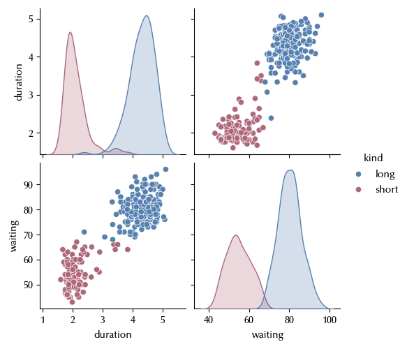
As we can see, both the duration and the waiting time depends on the kind of the geyser. We will now use a normal mixture model to fit the duration.

with pm.Model() as mix_model:
    sigma = pm.Gamma('sigma', alpha=1, beta=0.5, shape=2)
    mu = pm.Normal('mu', mu=2*np.arange(2), sigma=2, shape=2)
    pi = pm.Dirichlet('pi', a=np.ones(shape=2)/2.0)
    phi = pm.Normal.dist(mu=mu, sigma=sigma, shape=2)
    y = pm.Mixture('y', w=pi, comp_dists = phi, observed=geyser['duration'])

with mix_model:
        trace_mix = pm.sample(random_seed=rng, nuts_sampler='numpyro')

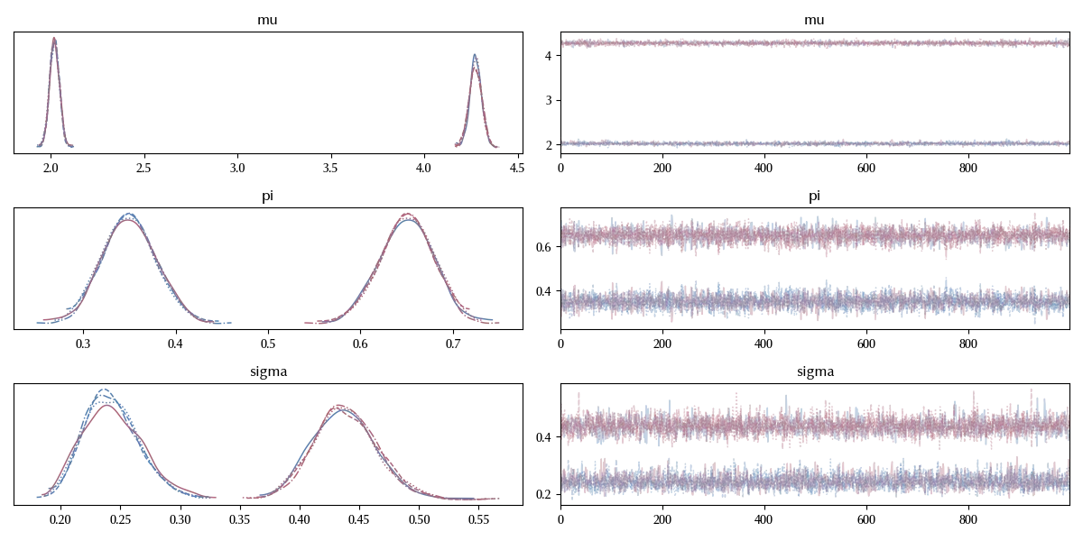
az.plot_trace(trace_mix)
fig = plt.gcf()
fig.tight_layout()

with mix_model:
    ppc_mix = pm.sample_posterior_predictive(trace_mix, random_seed=rng)

az.plot_ppc(ppc_mix, num_pp_samples=2000)

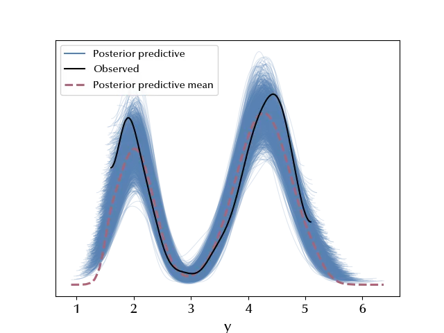
We can now use our model to classify an arbitrary geyser.

mu0 = trace_mix.posterior['mu'].values.reshape((-1, 2))[:, 0]
mu1 = trace_mix.posterior['mu'].values.reshape((-1, 2))[:, 1]
s0 = trace_mix.posterior['sigma'].values.reshape((-1, 2))[:, 0]
s1 = trace_mix.posterior['sigma'].values.reshape((-1, 2))[:, 1]
p0 = trace_mix.posterior['pi'].values.reshape((-1, 2))[:, 0]
p1 = trace_mix.posterior['pi'].values.reshape((-1, 2))[:, 1]

def f(d):
    x0 = (d-mu0)/s0
    x1 = (d-mu1)/s1
    l0 = scipy.stats.norm.pdf(x0)
    l1 = scipy.stats.norm.pdf(x1)
    h0 = np.mean(l0*p0)
    h1 = np.mean(l1*p1)
    return (h0/(h0+h1),h1/(h0+h1))

Let us now assume that we have observed two new geysers, and we want to know their kind. The first one has duration 2.8 and the second one 3.5.

f(2.8)

(0.5138327363599765, 0.48616726364002355)

f(3.5)

(1.2511916521712673e-06, 0.9999987488083479)

Therefore, it is slightly more probable that the first geyser is of type “short”, while the second one is of type “long” almost for sure.

Zero inflated models

Another very common kind of mixture model is the family of the zero-inflated model.

This kind of model becomes useful when you are dealing with count data, but you have an excess of zeros.

\[P(x | \theta, \omega) = \omega \delta_{x,0} + (1-\omega)P_0(x | \theta)\]

Let us use it on the fish dataset, from the UCLA repository

df = pd.read_csv('https://stats.idre.ucla.edu/stat/data/fish.csv')

sns.histplot(df, x='count')

We are dealing with a count dataset, and the number of zeros looks too large to be compatible with a Poisson or a negative binomial distribution.

with pm.Model() as inflated_model:
    w = pm.Beta('w', alpha=1, beta=1)
    mu = pm.Exponential('mu', lam=0.1)
    alpha = pm.Exponential('alpha', lam=1)
    y = pm.ZeroInflatedNegativeBinomial('y', psi=w, mu=mu, alpha=alpha, observed=df['count'])
    trace_inflated = pm.sample(chains=4, random_seed=rng, target_accept=0.9, nuts_sampler='numpyro')

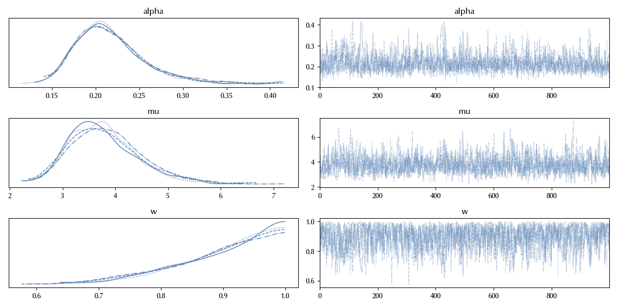
az.plot_trace(trace_inflated)

with inflated_model:
    ppc_inflated = pm.sample_posterior_predictive(trace_inflated, random_seed=rng)

r = ppc_inflated.posterior_predictive['y'].values.reshape(-1)

prob = [(r==k).astype(int).sum()/len(r) for k in range(r.max())]

fig = plt.figure()
ax = fig.add_subplot(111)
ax.hist(df['count'], alpha=0.8, bins=np.arange(30), density=True, color='gray')
sns.barplot(prob, ax=ax, fill=False, alpha=0.8)
ax.set_xlim([0, 30])
ax.set_xticks(np.arange(0, 30, 10))

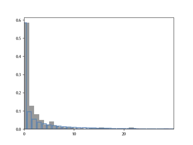
We didn’t use arviz because we got some issue due to the very large maximum number of count. From this figure it looks like the main behavior of the data is well captured by the model.

Conclusions

We discussed the family of the mixture models, and more in detail the normal mixture model and the zero-inflated model. We finally discussed how to implement them in PyMC and how to use a normal mixture model as a classifier.

%load_ext watermark

%watermark -n -u -v -iv -w -p xarray,pytensor,numpyro,jax,jaxlib

Last updated: Wed Nov 20 2024

Python implementation: CPython
Python version : 3.12.7
IPython version : 8.24.0

xarray : 2024.9.0
pytensor: 2.25.5
numpyro : 0.15.0
jax : 0.4.28
jaxlib : 0.4.28

seaborn : 0.13.2
matplotlib: 3.9.2
pymc : 5.17.0
numpy : 1.26.4
arviz : 0.20.0
pandas : 2.2.3
scipy : 1.14.1

Watermark: 2.4.3