Introduction to the linear regression

So far we discussed how to model one variable. With this post we will start a discussion on how to model the dependence of one variable on other variables, named covariates, regressors, predictors or risk factors depending on the research area we are dealing with.

Regression

In regression, we want to model the dependence of one variable $Y$ on one or more external variables $X$. In other words, we are trying to determine an $f$ such that

\[Y_i = f(X_i, \theta) + \varepsilon_i\]

where $\varepsilon_i$ is some random noise and $\theta$ represents a set of parameters. In the case of regression, we are not interested in modelling $X_i$. Notice that the distribution of the $Y_i$ is now different among different elements, as the parameters are assumed to depend on $X_i\,.$ In other words, the $Y_i$ are no more identically distributed. What we want to model is the statistical dependence, which is not an exact one, since we assume that there is some noise which makes our dependence inaccurate. This fact makes statistical dependence different from the mathematical dependence, where the relation is exactly fulfilled. We must also draw a distinction between statistical dependence and causal dependence, since a common misconception is that finding a statistical dependence implies a causal relation between $X$ and $Y$.

Causal inference requires much stronger assumptions than statistical inference.

We are only allowed to draw conclusions about causality when these assumptions are satisfied, as we will discuss later in this blog. Notice that referring to $X$ as the risk factor is usually done in the context of causal inference, and we will therefore avoid this term for now.

As pointed out by John Carlin in this paper, there are two main purposes for regression other than causal inference: we may either want to describe a relation between $X$ and $Y\,,$ or we may desire to use our model to predict the value of $Y$ one $X$ has been measured.

By Taylor expanding $f$ around $X=0$ we have that the simplest dependence we can assume is

\[Y_i = \theta_0 + \theta_1 X_i + \varepsilon_i\,,\]

we are therefore assuming the additivity of $Y_i$ with respect to $X_i\,.$

The assumption which is by far the most common for $\varepsilon_i$ is

\[\varepsilon_i \sim \mathcal{N}(0, \sigma)\]

We are therefore assuming that the errors are normally distributed, and that the variance is independent on $X_i\,.$ The constant variance assumption is named homoscedasticity, while the condition of variable variance is named heteroskedasticity.

Let us now take a look at our parameters:

$\theta_1$ is the average $Y$ difference of two groups with $\Delta Y = 1\,.$
$\theta_0$ is the intercept of the model. If our data includes $X=0$ we can interpret $\theta_0$ as the value of $Y$ when $X=0\,.$
$\sigma$ is the average variance.

GDP-Life expectancy relation

In order to understand our model, we will apply it to investigate the relation between the gross domestic product of a country and its life expectancy.

First of all, let us import the relevant libraries.

import requests
import json
import pandas as pd
import seaborn as sns
import numpy as np
import pymc as pm
import arviz as az
from matplotlib import pyplot as plt
from zipfile import ZipFile
import io

We can now download the GDP data from the IMF rest API as follows:

with requests.get('https://www.imf.org/external/datamapper/api/v1/NGDPDPC') as gdp:
    data_gdp = json.loads(gdp.content)

dt = {key: [data_gdp['values']['NGDPDPC'][key]['2021']]
        for key in data_gdp['values']['NGDPDPC'] if '2021' in data_gdp['values']['NGDPDPC'][key]}

df = pd.DataFrame.from_dict(dt).transpose().rename(columns={0: 'gdp'})

We also download the country names from the same API, and we combine the two tables

with requests.get('https://www.imf.org/external/datamapper/api/v1/countries') as countries:
    data_countries = json.loads(countries.content)

df_countries = pd.DataFrame.from_dict({key: [data_countries['countries'][key]['label']]
        for key in data_countries['countries']}).transpose().rename(columns={0: 'name'})

df_n = df.join(df_countries, how='inner')

The table containing the life expectancy can be downloaded from this page of the World Bank website. Rather than clicking on the website, we will download it automatically as follows

with requests.get('https://api.worldbank.org/v2/en/indicator/SP.DYN.LE00.IN?downloadformat=csv') as f:
    data = f.content
    z = ZipFile(io.BytesIO(data))

for name in z.namelist():
    if name.startswith('API'):
        dt = z.extract(name)
        df_lifexp = pd.read_csv(dt, skiprows=4)

We can now combine the two dataframes. We will stick to the year 2021, as it is the most recent year for most of the countries.

df_le = df_lifexp[['Country Code', '2021']].set_index('Country Code').dropna().rename(
    columns={'2021': 'Life expectancy'})

df_final = df_n.join(df_le, how='inner')

sns.pairplot(df_final)

The pairplot of our variables

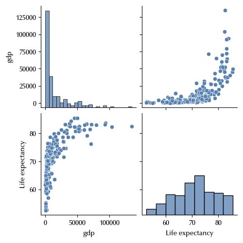
There appears to be no linear relation between the two. However, by a suitable variable redefinition, we can get linearity within a good approximation.

df_final['log GDP'] = np.log(df_final['gdp'])

sns.pairplot(df_final[['log GDP', 'Life expectancy']])

The pairplot of our variables

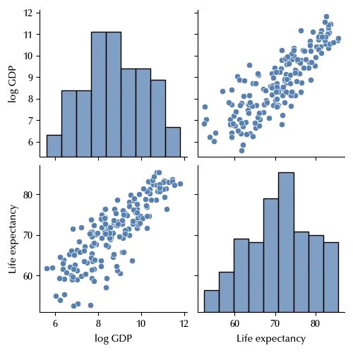
The homoscedasticity only seems to hold approximately, as in the region with lower GDP the data shows a larger variance with respect to countries with higher GDP. For the sake of simplicity, we will stick to the constant variance assumption, and we will see how to deal with heterogeneous variance in a future post.

Let us now set up our model

rng = np.random.default_rng(42)
x_pred = np.arange(5, 13, 0.1)

with pm.Model() as model:
    alpha = pm.Normal('alpha', mu=0, sigma=50)
    beta = pm.Normal('beta', mu=0, sigma=10)
    sigma = pm.HalfNormal('sigma', sigma=10)
    y = pm.Normal('y', mu=alpha+beta*df_final['log GDP'], sigma=sigma, observed=df_final['Life expectancy'])
    y_pred = pm.Normal('y_pred', mu=alpha+beta*x_pred, sigma=sigma)  # We want to get the error bands for all the values of x_pred

with model:
    trace = pm.sample(random_seed=rng, chains=4, draws=2000, tune=2000, nuts_sampler='numpyro')

az.plot_trace(trace, var_names=['alpha', 'beta', 'sigma'])
fig = plt.gcf()
fig.tight_layout()

The trace plot

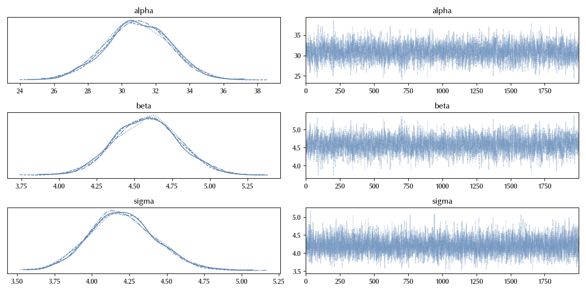
The trace looks fine. We will directly check the posterior predictive distribution.

with model:
    ppc = pm.sample_posterior_predictive(trace)

y_mean = trace.posterior['y_pred'].values.reshape((-1, len(x_pred))).mean(axis=0)
y_low = np.quantile(trace.posterior['y_pred'].values.reshape((-1, len(x_pred))), 0.025, axis=0)
y_high = np.quantile(trace.posterior['y_pred'].values.reshape((-1, len(x_pred))), 0.975, axis=0)

fig = plt.figure()
ax = fig.add_subplot(111)
ax.fill_between(x_pred, y_low, y_high, color='lightgray')
ax.plot(x_pred, y_mean, color='grey')
ax.scatter(df_final['log GDP'], df_final['Life expectancy'])
ax.set_xlim([np.min(x_pred), np.max(x_pred)])
ax.set_xlabel('Log GDP per Capita')
ax.set_title('Life Expectancy 2021')

The posterior predictive

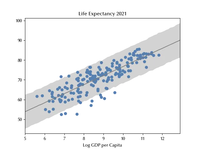
While our model correctly reproduces the relation between the GDP and the average life expectancy, it fails to reproduce the observed variance, confirming that the homoscedasticity assumption is violated.

Let us now inspect which nations show the biggest error

(df_final['Life expectancy'] - np.mean(trace.posterior['alpha'].values.reshape(-1))
- np.mean(trace.posterior['beta'].values.reshape(-1))*df_final['log GDP']).sort_values(ascending=True).head()

NGA -13.328530
SWZ -12.201977
GNQ -11.809278
NRU -11.197007
NAM -10.621142
dtype: float64

The above nations are Nigeria, eSwatini, Equatorial Guinea, Nuaru and Nambia, so it looks like our model fails to reproduce some African and Oceania countries, which have an average life expectancy much lower than non-African and non-Oceania countries with similar GDP.

Let us also check if the assumption about the normality of the deviation from the average trend is fulfilled within a good approximation

fig = plt.figure()
ax = fig.add_subplot(111)
ax.hist(
(df_final['Life expectancy'] - np.mean(trace.posterior['alpha'].values.reshape(-1)) 
 - np.mean(trace.posterior['beta'].values.reshape(-1))*df_final['log GDP']), bins=np.arange(-15, 10,1.5))
ax.set_title('Residuals histogram')

The pairplot of our variables

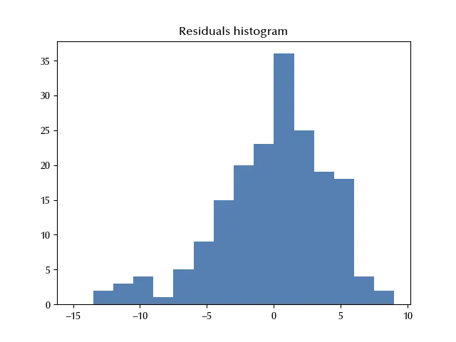
It appears that the distribution of the residual is left skewed, so in order to improve our model we could use a skewed distribution, like the Skewed Normal distribution or the Variance Gamma instead of a normal distribution.

This is however a somehow more advanced topic with respect to an introductory post on linear regression, so we won’t implement these models here.

Conclusions

We introduced the linear model, and we saw how to implement it with an example. As we will see in the future posts, the linear model is the starting point for almost any regression model. We discussed the interpretation of the parameters and some of the most relevant assumptions we made about data.

Regression

GDP-Life expectancy relation

Conclusions

Suggested readings