Linear regression with binary input
Linear regression can be straightforwardly applied when the independent variable $X$ is discrete. One should only pay attention to the interpretation of the parameters in this case, as the interpretation provided in the previous post may not apply.
The model
Here we will use the “Student alcohol consumption” dataset, available on this data.world page. In this study, the authors analyzed the relationship between alcohol consumption and many aspects of the student’s life, including the school behavior. We will analyze the difference in the math grades between male and female students.
Our model will be the following
\[y_i = \mathcal{N}(\mu_i, \sigma)\]where
\[\mu_i = \beta_0 + \beta_1 x_i\]and
\[x_i = \begin{cases} 0 & if\, x=F\\ 1 & if\, x=M \end{cases}\]In this case we have that, for female students, the average grade is $\beta_0\,,$ while for male students it is $\beta_0 + \beta_1\,.$
The female group and, more generally, the group with average dependent variable $\beta_0\,,$ is called the reference group.
The parameter $\beta_1$ can be now interpreted as the difference between the average male and female grade.
The implementation
Let us now see how to implement this model
import seaborn as sns
import pandas as pd
from matplotlib import pyplot as plt
import numpy as np
import pymc as pm
import arviz as az

df = pd.read_csv('https://query.data.world/s/qz5sf27veajjivl3bpa5npazsxzn7z?dws=00000')
Let us now only keep the columns we are interested in
df_red = df[['sex', 'G3']]

df_red['sex'] = df_red['sex'].astype('category')

df_red.head()
| sex | G3 | |
|---|---|---|
| 0 | F | 6 |
| 1 | F | 6 |
| 2 | F | 10 |
| 3 | F | 15 |
| 4 | F | 10 |
We can now easily build our model. We could easily do this as follows:
x = (df_red['sex']=='M').astype(int)
This method works fine for a binary category, but this method becomes cumbersome as the number of categories grows. Fortunately, pandas provides a builtin function to do this job, namely the “factorize” function.
x, cat_data = pd.factorize(df_red['sex'])

cat_data
Since the first category is “F”, the females will be associated to the 0 values in x, while males will be associated to 1.
We can now implement the model
rng = np.random.default_rng(42)
with pm.Model() as model:
    beta = pm.Normal('beta', mu=0, sigma=20, shape=(2))
    sigma = pm.HalfNormal('sigma', sigma=20)
    mu = beta[0] + beta[1]*x
    y = pm.Normal('y', mu=mu, sigma=sigma, observed=df_red['G3'])
    idata = pm.sample(nuts_sampler='numpyro', random_seed=rng)

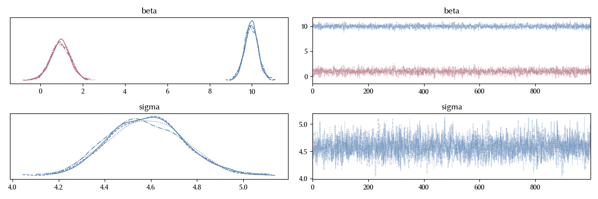
az.plot_trace(idata)
fig = plt.gcf()
fig.tight_layout()

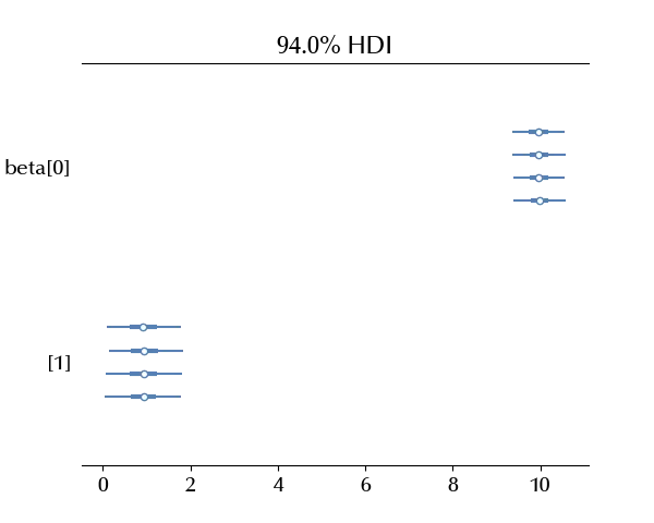
Let us take a better look to the beta parameters
az.plot_forest(idata, var_names='beta')

It looks like, in this study, the male students have on average a slightly higher math grade than the female students.
Posterior predictive checks
Let us now verify if the observed data are included within the predicted uncertainties
with model:
    ppc = pm.sample_posterior_predictive(idata, random_seed=rng)

fig = plt.figure()
ax = fig.add_subplot(111)
for yt in az.extract(ppc, num_samples=20, group='posterior_predictive')['y'].T:
    s = rng.uniform(low=-0.1, high=0.1, size=len(x))
    ax.scatter(x+s, yt, color='lightgray', s=5)
ax.scatter(x, df_red['G3'], s=5)
ax.set_xticks([0, 1])
ax.set_xticklabels(['F', 'M'])

In the above code block, we “jittered” (added a small random number to the x variable) in order to be able to distinguish the points.
The posterior predictive looks good, so we can conclude that on average the male students performed slightly better than the female ones. We could of course improve our model by imposing that the grade is non-negative, but if we simply want to investigate the mean difference, this model is enough for our purposes. We want to stress that this does not imply that being males makes you perform better at math with respect to females or vice versa, this would be wrong for many reasons. First of all, as we will discuss in the section about causal inference, this statement has no meaning in the counterfactual definition of causality, as you cannot manipulate someone’s biological sex.
Conclusions
We extended the linear regression model to a binary outcome, and discussed the interpretation of the parameter’s models when the binary regressor encodes a categorical variable.
%load_ext watermark
%watermark -n -u -v -iv -w -p xarray,pytensor,numpyro,jax,jaxlib
Python implementation: CPython
Python version : 3.12.7
IPython version : 8.24.0
xarray : 2024.9.0
pytensor: 2.25.5
numpyro : 0.15.0
jax : 0.4.28
jaxlib : 0.4.28
arviz : 0.20.0
pandas : 2.2.3
pymc : 5.17.0
numpy : 1.26.4
seaborn : 0.13.2
matplotlib: 3.9.2
Watermark: 2.4.3
