Trace inspection

In the last post we introduced the concept of Bayesian workflow. Starting from this post, we will discuss some of the most important aspects, and we will do so by starting with the trace assessment.

In this post I will not provide you the details of the computation, as our only purpose will be to look for pathologies into the trace. I will often exacerbate some issue to make the issues visible, and I will do this by means of really short traces or crazy parameters.

Tricking the NUTS sampler is not easy, but this may happen when your parameter space is large or has some bad structure. In this case, however, the issues overlap, and it is less clear how to handle them. For this reason I preferred to switch to simpler models but with bad parameter choices. I also used on purpose a quite small number of draws, as a larger one would make harder to spot by eye the pathologies.

Your enemy is the auto-correlation

When we compute the traces, we are trying a draw a sample of i.i.d. units from the posterior probability. We are however using a deterministic method to do so, where each draw depends on the previous one, we therefore have that our traces will be auto-correlated. For this reason, our main task will be to draw a set of stationary chains with a negligible auto-correlations.

Convergence not reached

The first kind of issue is usually very easy to spot, and it’s the non-stationary trace. In this case we didn’t left enough time to the sampler to reach the stationary regime, and in this case the trace shows a clear trend.

This happens because our algorithm started from a point which may be far away from the high density region, so we need some iteration to reach that region.

The solution, in this case, is quite clear: you should increase the number of tuning draws.

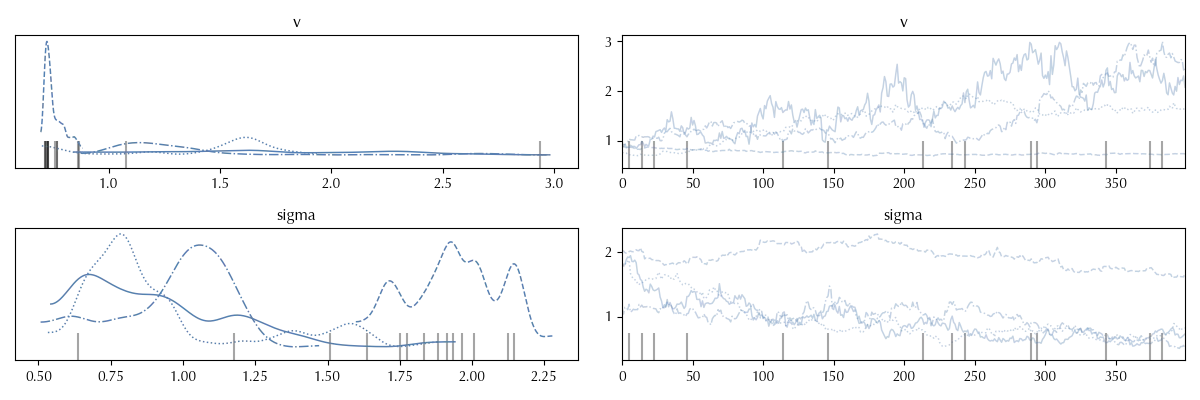
As we have already seen, the above plot can be done with Arviz’ plot_trace function.

Large autocorrelation

Let us take a look at a second trace.

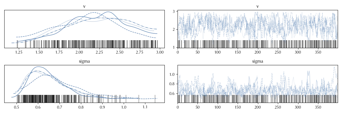
In this case the trace does not show any trend. There is however a very large auto-correlation. This can be seen on the right hand side of the plot, by observing that the trace is globally stationary, but locally the average is not constant (take a look at the $v$ variable around $i=150$, it is clearly visible some kind of bump).

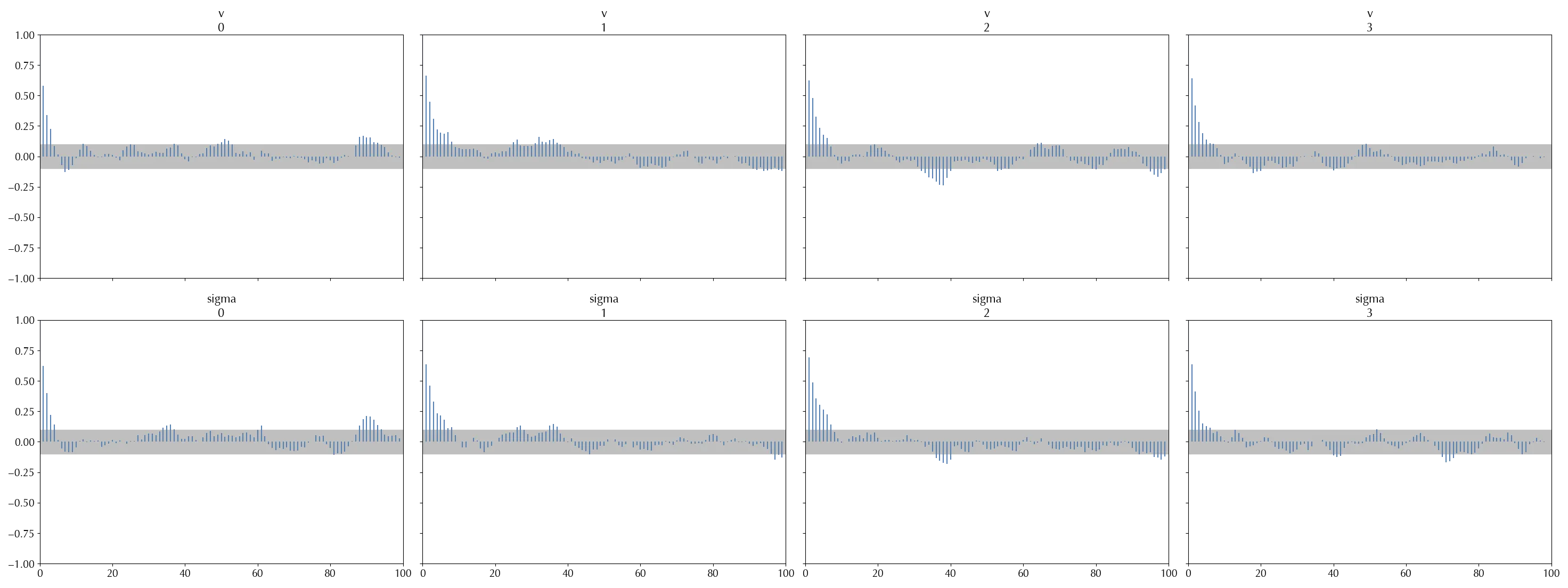
You can plot the autocorrelation by using the plot_autocorr function.

The ACF function

For a fixed-step time series $\{X_t\}_{t=1,...T}$ the auto-correlation function is defined es $$ \rho(\tau) = \mathbb{E}[\frac{(X_t-\mu)(X_{t+\tau}-\mu)}{\sigma^2}] $$ where $$ \mu = \mathbb{E}[X_t] $$ and $$ \sigma^2 = \mathbb{E}[(X_t-\mu)^2] \,. $$ By definition, $-1\leq \rho(t) \leq 1\,, \rho(0) = 1\,.$ Moreover, if the observations are i.i.d., we have that $ \rho(\tau>0)=0\,, $ since $$\mathbb{E}[(X_t-\mu)(X_{t+\tau}-\mu)] = \mathbb{E}[(X_t-\mu)]^2=(\mu-\mu)^2=0\,.$$
We can estimate $\rho(\tau)$ as $$ \begin{align} \rho(\tau) = & \frac{1}{T \sigma^2} \sum_{t=1}^T (X_t-\mu)(X_{t+\tau}-\mu)\\ \mu = & \frac{1}{T} \sum_{t=1}^T X_t \\ \sigma^2 = & \frac{1}{T} \sum_{t=1}^T (X_t-\mu)^2 \\ \end{align} $$

This kind of issue becomes clear when one plots the auto-correlation function with arviz. We can clearly see an oscillating behavior, as well as a very large asymptotic estimate for the upper bound of the coefficients.

The $\hat{R}$ statistics can help in spotting this kind of issue, as in these cases it generally differs from 1.

	mean	sd	hdi_3%	hdi_97%	mcse_mean	mcse_sd	ess_bulk	ess_tail	r_hat
v	2.193	0.389	1.531	2.921	0.024	0.017	268	520	1.02
sigma	0.662	0.103	0.506	0.845	0.008	0.006	238	290	1.03

We recall that the above table can be obtained by using the summary function.

The $\hat{R}$ statistics

The $\hat{R}$ exploits the fact that all our chains should be random sub-samples of a common distribution. Let us now indicate as $X^j_i$ the $i$th sample of the $j$th trace, where $i=1,...,S$ and $j=1,...,M\,.$ The variance is defined as $$ Var[X] = \frac{1}{M S-1}\sum_{j=1}^M \sum_{i=1}^S (X^j_i - \mu)^2 \approx \frac{1}{M S}\sum_{j=1}^M \sum_{i=1}^S (X^j_i - \mu)^2 $$ where $$ \mu =\frac{1}{M S}\sum_{j=1}^M \sum_{i=1}^S X^j_i $$ We can approximate the above quantity as the average within-variance $W$ $$ W = \frac{1}{M} \sum_{j=1}^M \sigma_j^2 $$ where $$ \sigma_j^2 = \frac{1}{S-1} \sum_{i=1}^S (X^j_i - \mu_j)^2 $$ and $$ \mu_j = \frac{1}{S} \sum_{i=1}^S X^j_i\,. $$ Notice that $$ \mu = \frac{1}{M} \sum_{j=1}^M \mu_j $$ We now define the between sample variance $B$ as $$ B = \frac{S}{M-1} \sum_{j=1}^M (\mu_j-\mu)^2 $$ We can estimate the variance as $$ Var[X] = \frac{S-1}{S} W + \frac{1}{S} B $$ $$ \begin{align} & \sum_{j=1}^M \sum_{i=1}^S (X^j_i - \mu)^2 = \sum_{j=1}^M \sum_{i=1}^S (X^j_i - \mu_j + \mu_j - \mu)^2\\ & = \sum_{j=1}^M \sum_{i=1}^S ( (X^j_i - \mu_j)^2 + (\mu_j - \mu)^2 +2 (X^j_i - \mu_j) (\mu_j - \mu)) = \sum_{j=1}^M \sum_{i=1}^S( (X^j_i - \mu_j)^2 + (\mu_j - \mu)^2 )\\ & = (S-1) M W + (M-1)B \leq (S-1) M W + M B \end{align} $$ We may therefore put an upper bound to the variance as $$ Var^+[X] = \frac{S-1}{S} W + \frac{B}{S} $$ This quantity is an unbiased estimator of the variance in the limit $S\rightarrow \infty$ as well as if stationarity holds, since in this case $B=0\,.$ The $\hat{R}$ statistics is defined as the square root of the ratio between the above quantity and the pooled variance $W$ $$ \hat{R} = \sqrt{\frac{Var^+[X]}{W}} \geq 1\,. $$

While in these cases the core part of the distribution is reliable enough, so you can safely estimate the mean, you should never trust to estimates involving peripheral regions of the posterior, like the $95\%$ HDI, unless your sample size is large enough.

In this case one should first try to leave to the sampler more time to find the optimal parameters. The NUTS sampler, by construction, tries to reduce the autocorrelation as much as possible in the tuning phase.

This may however be very difficult due some pathologies of the posterior distribution. As an example, this may happen if one parameter has a large posterior for very large values while for another one the optimal region is for very small values. This kind of problem becomes even worst when there is a large correlation between the parameters.

You should therefore try and re-parametrize your model. A simple rescaling in the parameters may be sufficient, but sometimes it is necessary to find a parametrization where the parameters are decoupled.

As an example, if your likelihood reads

\[Y \sim \mathcal{N}(\mu, \sigma)\]

you should consider rewriting it as

\[Y \sim \mu + \mathcal{N}(0, \sigma)\]

or you could even introduce an auxiliary random variable $X \sim \mathcal{N}(0, 1)$ and rewriting your model as

\[Y \sim \mu + \sigma X\]

Another possible solution is to use a smaller dataset, or to think if you are constraining too much or too little your parameters and change your prior accordingly.

The rank plot

Here we will deal with the same kind of issues that we have discussed above, but where the presence of the issue cannot be clearly seen with the above tools.

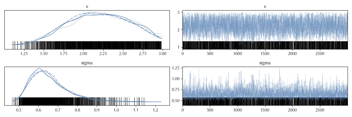
The above trace may look OK at a first glance, there is no clear auto-correlation pattern and the chains are quite similar. They are however not identical, and this should warn you.

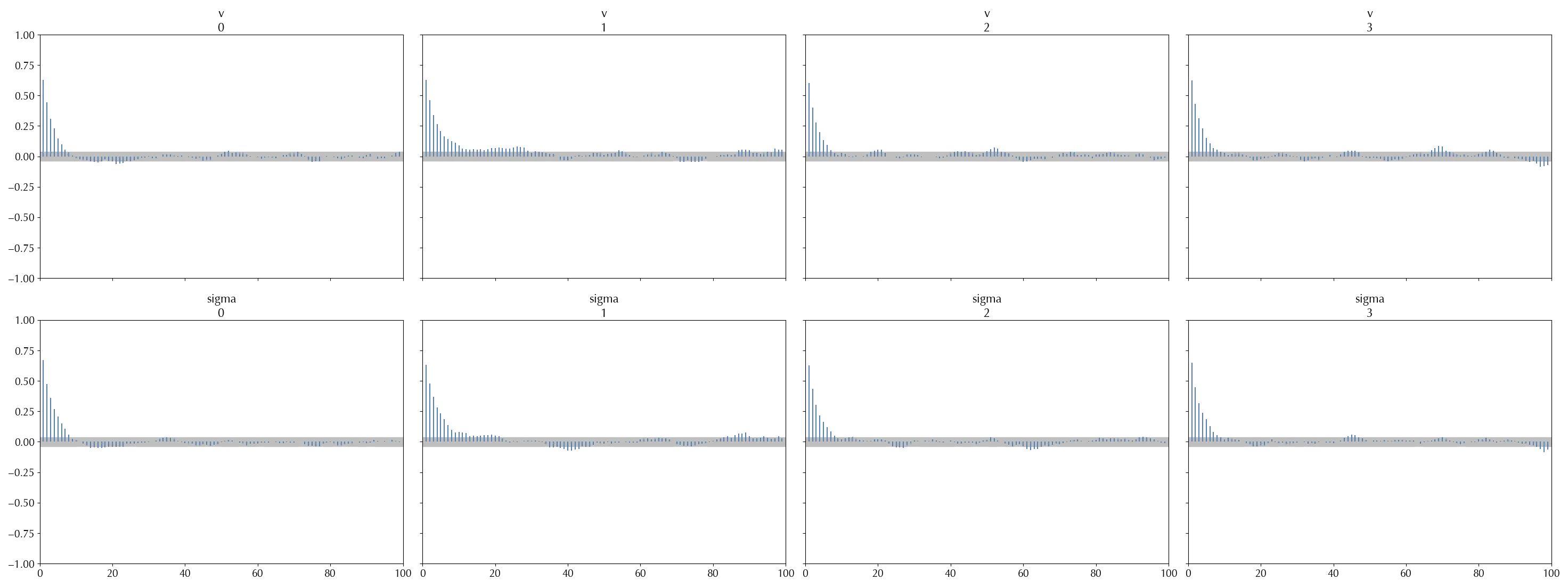
Also by looking at the auto-correlation plot it may be unclear if there is any issue.

	mean	sd	hdi_3%	hdi_97%	mcse_mean	mcse_sd	ess_bulk	ess_tail	r_hat
v	2.195	0.388	1.539	2.927	0.008	0.006	2162	2807	1
sigma	0.659	0.099	0.512	0.851	0.002	0.002	2307	2803	1

From the trace summary you would hardly guess that there is some issue, as the effective sample size is above 2000 and the $\hat{R}$ is one.

However, by looking at the rank plot, you can easily realize that there is something going on.

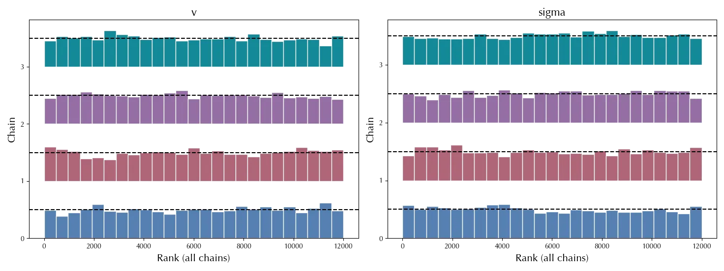
The rank plot

The rank plot is another tool to verify that all the chains are distributed according to the same distribution. In order to build the rank plot, given a set of equally spaced points $$\{ 0=z_0 < z_1 < \dots < z_n = 1 \}$$ You then compute the quantiles $q_k$ corresponding to the fraction $z_k$, and finally estimate the probability $$P(q_{k-1} \leq X^j < q_k)$$ for each chain $\{X^j_i\}_i$. By construction, the resulting distribution should be uniform, since the distribution of each chain should be the same of the combined chains. If it is not, it means that the chains are not distributed according to the same distribution, and you are facing some sampling issue.

In the above figure, the chain number $1$ of the variable $v$ shows some clear departure from the uniform distribution around $2000$, and the same happens for the second bar of the trace number $0\,.$

If you want a reliable estimate of the entire distribution, you should make sure that this kind of pattern is not visible. If this is the only issue, it is likely that a larger number of draws is sufficient.

Jumping traces

In some cases your model may be ill-defined, and it might happen that two subsets of parameters with different values can be exchanged without changing the probability. In these cases what might happen is that different chains of a parameter will converge to different values, as the case below.

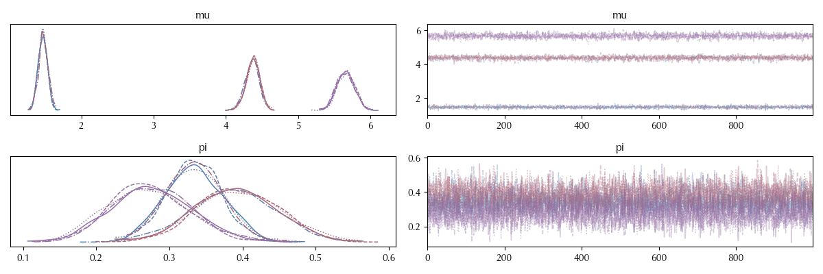
In order to better see this issue, let us take a look at the forest plot of the model.

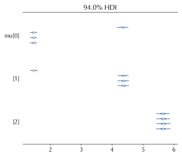
The estimate for $\mu_0$ from the 0-th chain is above 4, while the remaining chains are below 2. When we combine the four chains, of course, the estimate is totally unreliable

	mean	sd	hdi_3%	hdi_97%	mcse_mean	mcse_sd	ess_bulk	ess_tail	r_hat
mu[0]	2.186	1.256	1.34	4.444	0.624	0.478	7	29	1.53
mu[1]	3.649	1.261	1.399	4.539	0.626	0.479	7	29	1.53
mu[2]	5.66	0.123	5.438	5.887	0.003	0.002	2065	2125	1

This can be clearly seen by the crazy value of $\hat{R}\,,$ since the estimated variance from the combined chain is very different from the one estimated by combining the variances of the single chains.

In this case, the only safe solution is to re-parametrize your model, imposing an order to the parameters.

Conclusions

We have seen some of the most common kind of issues that you may encounter, some tools to diagnose these issues and some possible solutions. This is of course only a selected list, and you may encounter some other issues, especially when the model complexity grows. You should therefore always carefully inspect the trace to exclude issues which may affect your conclusions.