Predictive checks

In this post we will collect two different phases of the Bayesian workflow, namely the prior predictive checks and the posterior predictive checks.

The first one is aimed to ensure that your priors are compatible with the current domain knowledge, and it doesn’t require the comparison of the model prediction with the true data.

The posterior predictive checks, instead, are focused on clarifying if your fitted model can catch the relevant aspects of the data. You should always keep in mind that, even if it does a good job in describing the known data, this does not imply that the model will be successful in predicting future observations.

I believe that it is possible to learn from experience. That is where my faith comes in. And I think that all scientists who believe the same are consciously or unconsciously exercising an act of faith.

J. O. Irwin

While the two phases are in principle different, they use similar methods, and for this reason they are collected in a single post.

Prior predictive checks

When you are performing a prior predictive check, you are verifying if your model is flexible enough to include what you know about the problem and that you are implementing the appropriate constraints.

There are many ways you can perform this, and this can be done by generating fake data according to what you know about the problem and then fit them.

If you know nothing, you may decide to pick a dataset sub-sample and ensure that it is included within the prior predictive. Remember, however, that you do not want to fit the sub-sample, otherwise you may end up overfitting your data.

The twitter data again

Let us consider again the dataset introduced in the post on the Negative Binomial. We already discussed some checks in that post, and we carefully chose the value of the parameters by making an educated guess on the order of magnitude of the interactions.

Let us now assume that this time we made some error in the procedure and we take

\[\begin{align} \theta & \sim \mathcal{B}(1/2, 1/2)\\ \nu & \sim \mathcal{Exp}(20) \end{align}\]

It is not rare to mess up with the parametrization, so we may have confused $\lambda$ with its inverse (it is more common than what you may imagine). While the imported libraries and the data are the same, this time the model reads as follows

import pandas as pd
import numpy as np
import pymc as pm
import arviz as az
from matplotlib import pyplot as plt

df = pd.read_csv('./data/tweets.csv')

rng = np.random.default_rng(42)

with pm.Model() as pp0:
    nu = pm.Exponential('nu', lam=50)
    theta = pm.Beta('theta', alpha=1/2, beta=1/2)
    y = pm.NegativeBinomial('y', p=theta, n=nu, observed=yobs)

Let us now sample the prior predictive

with pp0:
    prior_pred_pp0 = pm.sample_prior_predictive(random_seed=rng)

fig = plt.figure()
ax = fig.add_subplot(111)
ax.hist(
prior_pred_pp0.prior_predictive['y'].values.reshape(-1), bins=np.arange(20), density=True)
ax.set_xlim([0, 20])

We can see that the value $y=0$ has a probability greater than the $90\%.$ Let us now compute this probability. This can be done by simply counting the fraction of sampled points equal to 0, and this can be done as follows:

(prior_pred_pp0.prior_predictive['y']==0).mean()

xarray.DataArray 'y'
array(0.97648148)

• Coordinates: (0)
• Indexes: (0)
• Attributes: (0)

It doesn’t really make much sense to start from a model which predicts that the $98\%$ of our tweets have zero interaction.

At this point, a wise Bayesian would go back and check again the model. Let us see what happens to the unwise Bayesian who fits the model despite the unreasonable conclusion which follows from the prior.

with pp0:
    trace_pp0 = pm.sample(random_seed=rng, chains=4, draws=5000, tune=2000, nuts_sampler='numpyro')

az.plot_trace(trace_pp0)
fig = plt.gcf()
fig.tight_layout()

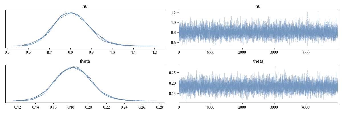
With the old model, the value of $\nu$ was peaked at $\nu = 2\,,$ while this time we have a peak at around $0.8\,.$ This means that our inference is strongly biased by our prior. In fact, our posterior predictive is much worse that the one in the old post.

with pp0:
    pp = pm.sample_posterior_predictive(trace_pp0, random_seed=rng)
az.plot_ppc(pp)

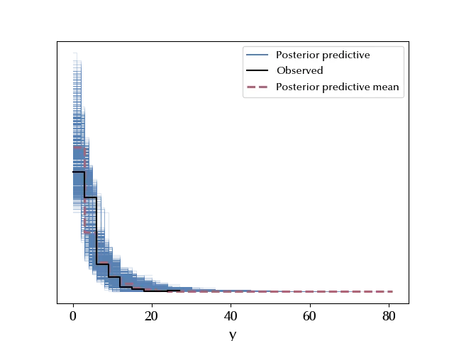
While our old model gave us, on average, the correct probability for the tweet with the lowest interaction number, this time we overestimate the number of tweets with few interactions.

Also in this case, the wise Bayesian would stop and go back to the model construction.

Conclusions

We discussed how to implement some prior predictive and posterior predictive check, together with the risks that comes by not doing them.

%load_ext watermark

%watermark -n -u -v -iv -w -p xarray,pytensor,numpyro,jax,jaxlib

Last updated: Wed Nov 20 2024

Python implementation: CPython
Python version : 3.12.7
IPython version : 8.24.0

xarray : 2024.9.0
pytensor: 2.25.5
numpyro : 0.15.0
jax : 0.4.28
jaxlib : 0.4.28

pymc : 5.17.0
numpy : 1.26.4
matplotlib: 3.9.2
arviz : 0.20.0
pandas : 2.2.3

Watermark: 2.4.3