The Negative Binomial model

In the last post we discussed the simplest model for count data, namely the Poisson model. Sometimes this model is not flexible enough, as in the Poisson distribution the variance is fixed by the mean. If your data is over-dispersed (or under-dispersed) the Poisson model might be not appropriate. This usually happens when your data cannot be treated as sampled according to an iid set of random variables. This often happens, as an example, with dataset coming from social networks, where each post has its own probability of interaction, depending on the topic but also on the algorithm modifications during the time. In this post I will explain how to deal with this kind of data by using the Negative Binomial model.

Trying with the Poisson model

I downloaded my own twitter data from analytics.twitter.com, and I wanted to analyze what’s the distribution of interaction rates across my tweets, and here’s the results ¹.

interactions	count
0	29
1	36
2	33
3	28
4	24
5	25
6	13
7	6
8	3
9	4
10	6
11	2
12	2
14	2
16	2
25	1

we can now check if the Poisson model does a good job in fitting the data. As before we will assume an exponential model for the Poisson mean, but since we have a larger average we choose $\lambda=1/50$ for the exponential parameter.

import pandas as pd
import numpy as np
import pymc as pm
import arviz as az
from matplotlib import pyplot as plt

df = pd.read_csv('./data/tweets.csv')

rng = np.random.default_rng(42)

yobs = df['interactions']

with pm.Model() as poisson:
    mu = pm.Exponential('mu', lam=1/50)
    y = pm.Poisson('y', mu=mu, observed=yobs)
    trace = pm.sample(random_seed=rng, chains=4, draws=5000, tune=2000, nuts_sampler='numpyro')

az.plot_trace(trace)

The trace seems OK, and for the sake of brevity we won’t perform all the trace checks. However, keep in mind that you should always do them. To compute the trace, we used the numpyro sampler, which is much faster than the ordinary NUTS sampler.

Let us jump to the posterior predictive check and verify if our model is capable to reproduce the data.

with poisson:
    ppc = pm.sample_posterior_predictive(trace, random_seed=rng)
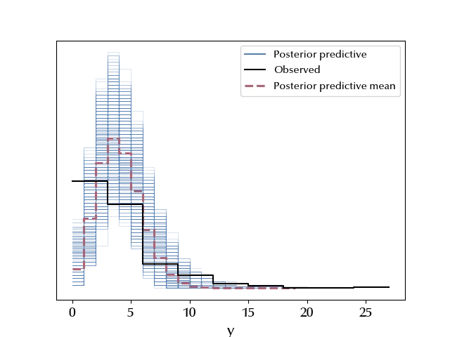
az.plot_ppc(ppc)

The average value doesn’t look at all like the observed points, and the error bands fail to include the data. This is definitely not a suitable model for our data.

The Negative Binomial model

We will now try and build a model with a Negative Binomial likelihood. According to Ockham’s razor principle, since the new model will have one more parameter than the previous one, in order to justify the increased model complexity, we should observe a clear improvement in the performances.

The new model assumes

\[Y \sim \mathcal{NegBin}(\theta, \nu)\]

The negative binomial distribution

Given a set of i.i.d. Bernoulli random variables $X_i$ having success probability $p\,,$ the negative binomial model describes the number of failures $x \in \mathbb{N}$ before you get a fixed number of successes $n>0\,.$ $$ p(x | n, p) \propto p^n (1-p)^x $$ We must now count the number of possible ways to rearrange the events. The last event is, by construction, a success. Therefore, we have that the number of possible ways to get $x$ failures out of $n+x-1$ events is $\binom{n+x-1}{x}\,,$ so $$ p(x | n, p) = \binom{x+n-1}{x} p^n (1-p)^x\,. $$ The parameter $n$ should, in principle, be integer. We can however extend the definition of the negative binomial distribution by means of the Gamma function $$ p(x | n, p) = \frac{\Gamma(x+n)}{\Gamma(x+1)\Gamma(n)} p^n (1-p)^x\,. $$ The parameter $p$ must belong to the $[0, 1]$ interval, and it can be parametrized as $$ p = \frac{\mu}{\mu+n} \,, \mu \geq 0\,. $$ When $n=1$ the negative binomial is also known as the geometric distribution, and this distribution has $$ p(x | p) = p (1-p)^x\,. $$ This distribution has expected value $$ \begin{align} \mathbb{E}_{geom}[X] = & \sum_{x=0}^\infty x p (1-p)^x = p \left(\sum_{x=1}^\infty x q^x\right)_{q=1-p} = p \left(q \sum_{x=0}^\infty x q^{x-1}\right)_{q=1-p} \\ = & p \left(q \frac{\partial}{\partial q} \sum_{x=0}^\infty q^{x}\right)_{q=1-p} = p \left(q \frac{\partial}{\partial q} \frac{1}{1-q} \right)_{q=1-p} = p \left( \frac{q}{(1-q)^2}\right)_{q=1-p} \\= & p \frac{1-p}{p^2} = \frac{1-p}{p} \end{align} $$ Since the negative binomial with a general $n$ can be seen as the sum of $n$ independent geometric random variables, it is straightforward to get $$ \mathbb{E}[X] = n \frac{1-p}{p}\,. $$ In the same way we can calculate $$ Var[X] = n \frac{1-p}{p^2}\,. $$

The above distribution, in PyMC, has more than one parametrization, but we will stick to the one already introduced, where $\theta \in [0, 1]$ and $\nu > 0\,.$

Since we want our guess for the parameters, we will assume

\[\theta \sim \mathcal{U}(0, 1)\]

We also expect $\nu$ to be somewhere between 1 and 10, as it should be roughly of the same order of magnitude of the mean of the observed data. Taking a mean $Y$ of 5 and $p=1/2$ we would have

\[10 = \nu \frac{1/2}{1-1/2} = \nu\]

so a reasonable assumption could be

\[\nu \sim \mathcal{Exp}(1/10)\]

We can now implement our model and verify if the trace has any problem.

with pm.Model() as negbin:
    nu = pm.Exponential('nu', lam=1/10)
    theta = pm.Uniform('theta')
    y = pm.NegativeBinomial('y', p=theta, n=nu, observed=yobs)
    trace_nb = pm.sample(random_seed=rng, chains=4, draws=5000, tune=2000, nuts_sampler='numpyro')

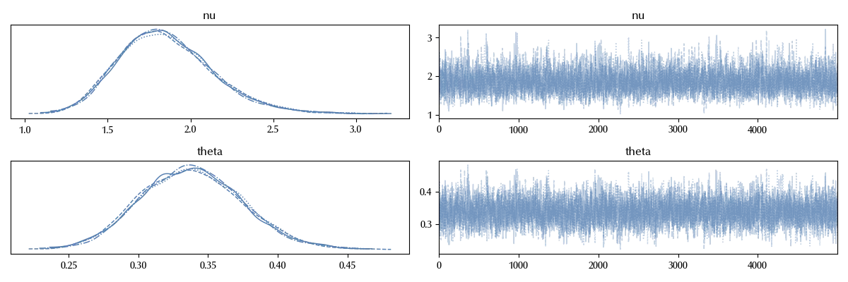
az.plot_trace(trace_nb)
fig = plt.gcf()
fig.tight_layout()

So far so good, so let us check the performances of the new model in reproducing the data.

with negbin:
    ppc_nb = pm.sample_posterior_predictive(trace_nb, random_seed=rng)
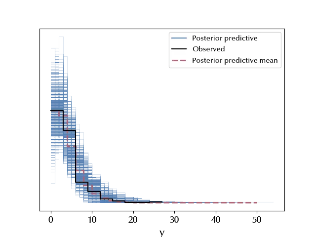
az.plot_ppc(ppc_nb)

The posterior predictive looks way better than the Poisson one.

A visual inspection is fundamental in checking the performances of posterior predictive distribution in reproducing the data. We can however use a very popular tool to have some additional information. We will use the Leave One Out cross validation. This technique, which uses the Pareto smoothed importance sampling, is equivalent to removing each datum and verifying how unlikely is the removed point with according to the new model. If the point is not too unlikely to appear, then the model is appropriate in reproducing the data, otherwise you may consider to look for a new model. This comparison requires the computation of the log likelihood, and the entire procedure can be done as follows

with poisson:
    pm.compute_log_likelihood(trace)

with negbin:
    pm.compute_log_likelihood(trace_nb)

df_comp_loo = az.compare({"poisson": trace, "negative binomial": trace_nb})

az.plot_compare(df_comp_loo)

This method confirms our conclusions, the Negative Binomial model performs better than the Poisson one.

Conclusions

We have discussed the Negative Binomial model and introduced the LOO method to perform a model comparison. We also saw in which situations it might be appropriate to choose a Negative Binomial model over a Poisson one.

%load_ext watermark

%watermark -n -u -v -iv -w -p xarray,pytensor,numpyro,jax,jaxlib

Last updated: Wed Nov 20 2024

Python implementation: CPython
Python version : 3.12.7
IPython version : 8.24.0

xarray : 2024.9.0
pytensor: 2.25.5
numpyro : 0.15.0
jax : 0.4.28
jaxlib : 0.4.28

matplotlib: 3.9.2
pandas : 2.2.3
arviz : 0.20.0
numpy : 1.26.4
pymc : 5.17.0

Watermark: 2.4.3

1. This happened when Twitter was a decent platform, and you could access your own statistics. ↩