The Poisson model
The last time we saw how to estimate probabilities. In this post we will take a first look at how to describe count data, i.e. non-negative integers. We will also anticipate the Bayesian workflow, which are the steps you should follow in order to ensure that your model is appropriate for your data. These steps will be discussed more in depth in a future section.
Clicks on a button
In one of the projects I have been working on, I have been asked to estimate the average number of clicks on a certain button in order to understand whether people used it and how. We already knew that it was not a very frequent event, we only expected a very small number of click per week. In this kind of situation, a common and appropriate choice is the Poisson model for the count data.
The Poisson distribution
The Poisson distribution is probably the simplest distribution for count data. Let us assume that we have an event that, on average, occurs $\mu>0$ times within a time $t\,.$ If every event is independent on the others, the probability that we observe $k$ events must go as $$P(X=k | \mu) \propto \frac{\mu^k}{k!}$$ where the denominator has been introduced since we don't care the order of the events. We can normalize it by observing that $$ \sum_{k=0}^\infty \frac{\mu^k}{k!} = e^\mu $$ therefore $$ p(k | \mu) =e^{-\mu } \frac{ \mu ^k}{k!}\,.$$ We have $$ \begin{align} \mathbb{E}[X] & = e^{-\mu} \sum_{k=0}^\infty k \frac{\mu^k}{k!} \\ & =e^{-\mu} \sum_{k=1}^\infty k \frac{\mu^k}{k!} \\ & =e^{-\mu} \sum_{k=1}^\infty \frac{\mu^k}{(k-1)!} \\ & =\mu e^{-\mu} \sum_{k=1}^\infty \frac{\mu^{k-1}}{(k-1)!} \\ & =\mu e^{-\mu} \sum_{k=0}^\infty \frac{\mu^{k}}{k!} \\ & = \mu \end{align} $$ Analogously we can obtain $$ Var[X] = \mathbb{E}[X^2] - \mathbb{E}[X]^2 = \mu $$The Poisson distribution requires a positive parameter $\mu\,,$ and since we are doing Bayesian inference, we must specify the prior distribution for this parameter.
The exponential and the gamma distribution
The exponential distribution is the simplest distribution for a positive real random variable, and its pdf reads $$ p(x | \lambda) = \lambda e^{-\lambda x}, \lambda > 0\,. $$ An exponentially distributed random variable $X$ with parameter $\lambda$ has expected value $$ \mathbb{E}[X] = \lambda \int_0^\infty dx x e^{-\lambda x} = \frac{1}{\lambda} $$ In a similar way we can obtain $$ Var[X] = \frac{1}{\lambda^2}\,. $$ Since this distribution is often considered too restrictive, you may decide and use the gamma distribution, which is a flexible generalization of the exponential distribution. $$ p(x | \alpha, \beta) = \frac{\beta^\alpha}{\Gamma(\alpha)} x^{\alpha -1} e^{-\beta x} $$ where $\alpha, \beta > \,.0$ For this distribution we have $$ \begin{align} \mathbb{E}[X] = & \int_0^\infty x \frac{\beta^\alpha}{\Gamma(\alpha)} x^{\alpha -1} e^{-\beta x} =\frac{\beta^\alpha}{\Gamma(\alpha)} \frac{1}{\beta^{\alpha+1}}\int_0^\infty dy y^{\alpha}e^{-y} = \frac{\beta^\alpha}{\Gamma(\alpha)} \frac{\Gamma(\alpha+1)}{\beta^{\alpha+1}} =\frac{\alpha}{\beta} \end{align} $$ Analogously $$ Var[X] = \frac{\alpha}{\beta^2} $$We will stick to the simplest possible distribution for $\mu\,,$ namely the exponential distribution. It is an appropriate distribution as it allows for any non-negative value, and it only has one parameter. We don’t think that, on average, the button has been clicked more than 10 times per week, so we can choose an average for the prior equal to 10:
\[\begin{align} y & \sim \mathcal{Poisson}(\mu) \\ \mu & \sim \mathcal{Exp}(1/10) \end{align}\]For the sake of completeness, here I report the number of occurrences of each count.
| count | number |
|---|---|
| 0 | 2 |
| 1 | 11 |
| 2 | 16 |
| 3 | 17 |
| 4 | 14 |
| 5 | 11 |
| 6 | 6 |
| 7 | 2 |
| 8 | 2 |
| 9 | 1 |
| 10 | 1 |
| >10 | 0 |
import pandas as pd
import pymc as pm
import arviz as az
from matplotlib import pyplot as plt

df = pd.read_csv('./data/clicks.csv')

df.head()
| week | count |
|---|---|
| 0 | 1 |
| 1 | 2 |
| 2 | 3 |
| 3 | 5 |
| 4 | 3 |
rng = np.random.default_rng(seed=42)

with pm.Model() as poisson:
    mu = pm.Exponential('mu', lam=0.1)
    y = pm.Poisson('y', mu=mu, observed=df['count'])

with poisson:
    trace = pm.sample(random_seed=rng, chains=4, draws=5000, tune=2000)
Above we specified that we want to draw four independent chains, to drop out the first 2000 samples from each trace and then to draw other 5000 samples for each trace. We need to drop out the first part of the trace because the sampler may start far away from a region with a high posterior distribution, and it might take a while to reach a higher density region. In this first phase, the sampling might not be distributed according to the desired distribution, and including it may introduce a bias into our estimates. Moreover, since the sampling algorithm is adaptive, we are allowing it to reach the optimal parameter (in the “true” sampling phase we must keep the parameters fixed in order to ensure a correct sampling).
A rule of thumb says that we should drop out the first 50% of the draws. This of course applies if you don’t have any idea about the convergence of the sampler, but since I already know that, for such a simple problem usually PyMC takes less than 1000 iterations to converge, I will take a slightly conservative number of draws equal to 2000.
The number of chains to sample is another crucial parameter, and its minimum recommended number is four. The reason for this is that one of the best ways to assess the convergence (or, to be more precise, to assess the presence of issues, as you can never be sure that there are no issues) is to compare different chains and verify that they are sampled according to the same distributions.
Trace diagnostics
Let us start checking if there is any issues.
az.plot_trace(trace)

As we can see, the trace seems stationary within a good approximation. There are neither regions where the trace is stuck (the sampling line is flat), so at a first visual inspection the trace looks fine.
Let us take a look at the trace summary
az.summary(trace)
| mean | sd | hdi_3% | hdi_97% | mcse_mean | mcse_sd | ess_bulk | ess_tail | r_hat | |
|---|---|---|---|---|---|---|---|---|---|
| mu | 3.502 | 0.205 | 3.143 | 3.909 | 0.002 | 0.002 | 7765 | 9168 | 1 |
As we previously mentioned, the ESS provides an estimate of the sampling error. In particular, it provides an estimate of the error due to the sampling auto-correlation which, ideally, should be zero. The exact meaning of it will be discussed in a future post, for now I only leave this explanation in the Stan website. As explained in this R documentation page, the MCSE is simply the standard deviation of the estimate (of the mean or of the standard deviation itself) divided by the ESS.
As explained in this preprint, the $\hat{R}$ statistics is recommended as the primary convergence diagnostic, and it has to be as closer to one as possible. Long story short, this statistics uses two different ways to provide an unbiased estimate of the variance of different chains. Ideally, they should be identical, so their ratio $\hat{R}$ should be equal to one. This diagnostic takes into account much more information than the ESS, as it compares different traces, and this is why it should be preferred to it. The number of chains should be at least four in order to provide a reliable estimate of this quantity.
As previously mentioned, the auto-correlation reduces the effective sample size. We can visually inspect the auto-correlation coefficients via
az.plot_autocorr(trace)
fig = plt.gcf()
fig.tight_layout()

The coefficients rapidly drop to 0, and this is the desired behavior. The gray band provide an estimate of the bounds for the auto-correlation coefficients of order higher than the calculated ones, and they are very small.
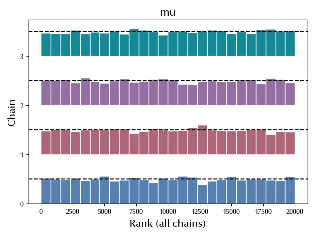
Another useful visual check that can be performed is the rank plot, where the posterior draw of each chain is ranked according to the combined posterior of the combined chains. If the chains are sampled according to the same distribution, then one should get a uniform distribution.
az.plot_rank(trace)
fig = plt.gcf()
fig.tight_layout()

As we can see, the distribution is quite consistent with the uniform distribution, so it doesn’t look like there are issues from this diagnostic.
Posterior predictive checks
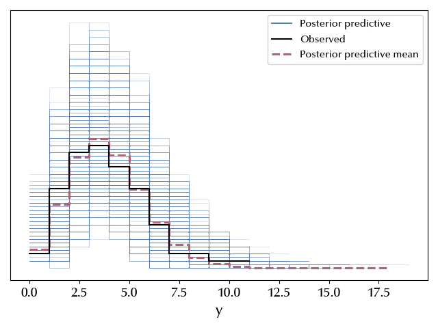
We can finally verify that our model is able to reproduce the data, and this is one of the most important checks that you should always do. For simple models like this one, it is sufficient to sample and plot the posterior predictive distribution. If the sampled distribution resembles the observed data and the error bars are big enough to accommodate the observed data, in this case is enough. For more complicated models, it might however be a good idea to perform additional checks.
with poisson:
    ppc = pm.sample_posterior_predictive(trace, random_seed=rng)

az.plot_ppc(ppc)
fig = plt.gcf()
fig.tight_layout()

The mean is really close to the observed one, and the data are well inside the estimated error bands, so we can safely assess that the model is appropriate to describe the data.
Conclusions
We discussed how to build a model for count data. We also introduced and briefly explained some of the most important checks one should do when using MCMC to make Bayesian inference.
%load_ext watermark
%watermark -n -u -v -iv -w
Python implementation: CPython
Python version : 3.12.7
IPython version : 8.24.0
xarray : 2024.9.0
pytensor: 2.25.5
numpyro : 0.15.0
jax : 0.4.28
jaxlib : 0.4.28
pandas : 2.2.3
matplotlib: 3.9.2
arviz : 0.20.0
pymc : 5.17.0
numpy : 1.26.4
Watermark: 2.4.3
