Re-parametrizing your model
Model re-parametrization is a part of the Bayesian workflow that will likely face any advanced user. On the other hand, if you are facing Bayesian inference for the first time, you might safely skip this (rather technical) post, which is about advanced concepts in MCMC.
When you will encounter this problem
The NUTS sampler is an amazing tool, but it is of course not perfect, and there are circumstances when even this tool has some issue. This is especially true in high dimensional, multiscale and highly correlated problems, where moving into the high density region of the posterior probability requires moving in a non-trivial space. A typical, well known class of models where this is likely to happen is the family of multilevel (or hierarchical) models, where even for a moderately high number of variables the sample space might become troublesome. Here we will re-phrase into the PyMC language this post . which discusses the same issue when dealing with Stan.
Fitting the Efron-Morris dataset
Here we will analyze the well known “batting average” Efron-Morris dataset, which can be found here
import pandas as pd
import pymc as pm
import arviz as az
import numpy as np
import seaborn as sns
from matplotlib import pyplot as plt

rng = np.random.default_rng(42)

df = pd.read_csv('https://raw.githubusercontent.com/pymc-devs/pymc4/master/notebooks/data/efron-morris-75-data.tsv', sep='\t')
In order to fit this dataset we will use a hierarchical model for the log-odds, similar to the one discussed here.
with pm.Model() as centered_logit_model:
    mu = pm.Normal('mu', mu=0, sigma=3)
    sigma = pm.HalfNormal('sigma', sigma=3)
    log_sigma = pm.Deterministic('log_sigma', pm.math.log(sigma))
    alpha = pm.Normal('alpha', mu=mu, sigma=sigma, shape=len(df))
    theta = pm.invlogit(alpha)
    y = pm.Binomial('y', observed=df['Hits'], n=df['At-Bats'], p=theta)

with centered_logit_model:
    idata_centered = pm.sample(nuts_sampler='numpyro', random_seed=rng)
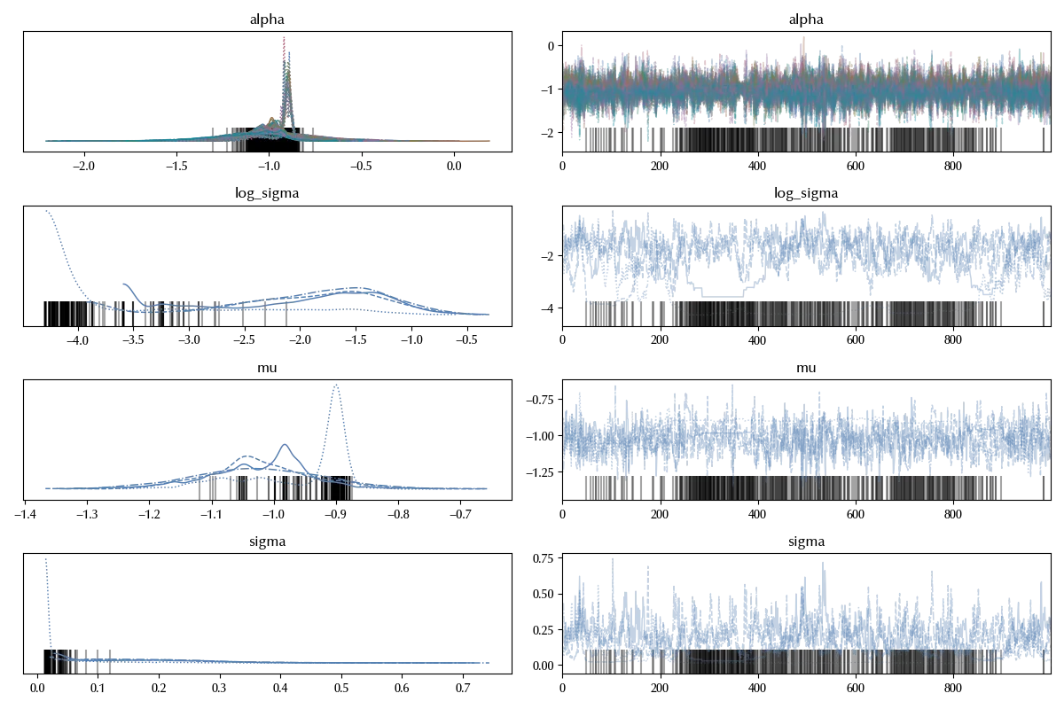
By running this code I got 517 divergences, and these terrible traces
az.plot_trace(idata_centered)
fig = plt.gcf()
fig.tight_layout()

As discussed in this paper, this is a common issue in hierarchical models. We can however circumvent this issue by observing that, if
\[\alpha_i \sim \mathcal{N}(\mu, \sigma)\]then we can rewrite the above as
\[\alpha_i = \mu + \sigma \phi_i\]where
\[\phi_i \sim \mathcal{N}(0, 1)\]with pm.Model() as noncentered_logit_model:
mu = pm.Normal('mu', mu=0, sigma=3)
sigma = pm.HalfNormal('sigma', sigma=3)
log_sigma = pm.Deterministic('log_sigma', pm.math.log(sigma))
alpha_std = pm.Normal('alpha_std', mu=0, sigma=1, shape=len(df))
alpha = pm.Deterministic('alpha', mu+sigma*alpha_std)
theta = pm.invlogit(alpha)
y = pm.Binomial('y', observed=df['Hits'], n=df['At-Bats'], p=theta)
with noncentered_logit_model:
idata_noncentered = pm.sample(nuts_sampler='numpyro', random_seed=rng)
az.plot_trace(idata_noncentered)
fig = plt.gcf()
fig.tight_layout()

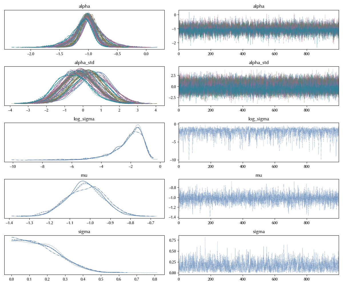
This is by far way better than the centered parametrization, and it worked so well because now our variables are well separated. Thanks to the re-parametrization, the sampling space is isotropic within good approximation, and it is therefore easier for the NUTS sampler to explore it. We can also take a look at the different landscapes in the $\mu-\sigma$ plane
az.plot_pair(idata_centered, var_names=['mu', 'log_sigma'])

az.plot_pair(idata_noncentered, var_names=['mu', 'log_sigma'])

As we can see, the centered parametrization had problems in exploring the region with a lower probability density, while the non-centered one also explored this region.
Conclusions
We discussed how model re-parametrization greatly improved the MCMC sampling procedure, by allowing you to sample clean traces even for highly correlated models.
%load_ext watermark
%watermark -n -u -v -iv -w -p xarray,pytensor,numpyro,jax,jaxlib
Python implementation: CPython
Python version : 3.12.7
IPython version : 8.24.0
xarray : 2024.9.0
pytensor: 2.25.5
numpyro : 0.15.0
jax : 0.4.28
jaxlib : 0.4.28
numpy : 1.26.4
pymc : 5.17.0
pandas : 2.2.3
seaborn : 0.13.2
arviz : 0.20.0
matplotlib: 3.9.2
Watermark: 2.4.3
