Model comparison
In the majority of cases, you won’t deal with a single model for one dataset, but you will try many models at the same time.
In this phase of the Bayesian workflow we will discuss some methods to compare models.
Comparing model sometimes may be understood as choosing the best model, but in most cases it means to assess which model is better to describe or predict some particular aspect of your data. Model comparison can be done analytically in some case, but most of the time it will be done numerically or graphically, and here we will give an overview of the most important tools.
Since all models are wrong the scientist must be alert to what is importantly wrong. It is inappropriate to be concerned about mice when there are tigers abroad.
George Box
Here we will take a look at two of the most important methods, the Bayes factor analysis and the Leave One Out cross-validation.
Bayes factors
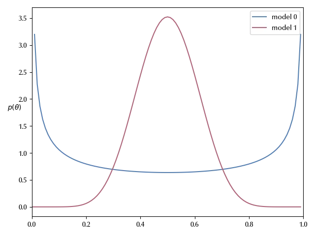
Let us go back to the Beta-Binomial model that we discussed in this post, and let us assume that we have two candidate models to describe our data: model 0 has Jeffreys prior, which mean that the prior is a beta distribution with $\alpha=1/2$ and $\beta=1/2\,.$ The second model, named “model 2”, is instead centered in $0.5$ and has \(\alpha = \beta = 10\,.\)
import numpy as np
from matplotlib import pyplot as plt
import pymc as pm
import arviz as az
from scipy.stats import beta

y = 7
n = 4320

model_0 = {'a': 1/2, 'b': 1/2}
model_1 = {'a': 10, 'b': 10}

x_pl = np.arange(0, 1, 0.01)
fig = plt.figure()
ax = fig.add_subplot(111)
for k, model in enumerate([model_0, model_1]):
    ax.plot(x_pl, beta(a=model['a'], b=model['b']).pdf(x_pl), label=f"model {k}")
legend = plt.legend()
ax.set_ylabel(r"$\theta$")
ax.set_ylabel(r"$p(\theta)$  ", rotation=0)
ax.set_xlim([0, 1])
fig.tight_layout()

Given the two models $M_0$ and $M_1$ we may ask which one we prefer, given the data. The probability of the model given the data is given by
\[p(M_k | y) = \frac{p(y | M_k)}{p(y)} p(M_k)\]where the quantity
\[p(y | M_k)\]is the marginal likelihood of the model.
If we assign the same prior probability $p(M_k)\,,$ to each model, since $p(y)$ is the same for both models, then we can simply replace $p(M_k | y)$ with the marginal likelihood.
As usual, an analytic calculation is only possible in a very limited number of models.
One may think to compute $p(M_k| y)$ by starting from $p(y | \theta, M_k)$ and integrating out $\theta$ but doing this naively is generally not a good idea, as this method is unstable and prone to numerical errors.
We can however use the Sequential Monte Carlo to compare the two models, since it allows to estimate the (log) marginal likelihood of the model.
models = []
traces = []

for m in [model_0, model_1]:
    with pm.Model() as model:
        theta = pm.Beta("theta", alpha=m['a'], beta=m['b'])
        yl = pm.Binomial("yl", p=theta, n=n, observed=y)
        trace = pm.sample_smc(1000, return_inferencedata=True, random_seed=np.random.default_rng(42))
        models.append(model)
        traces.append(trace)
Let us inspect as usual the traces.
az.plot_trace(traces[0])

az.plot_trace(traces[1])

What one usually computes is the Bayes factor of the models, which is the ratio between the posterior probability of the model (which in this case is simply the ratio between the marginal likelihoods).
| $BF = p(M_0)/p(M_1)$ | interpretation |
|---|---|
| $BF<10^{0}$ | support to $M_1$ (see reciprocal) |
| $10^{0}\leq BF<10^{1/2}$ | Barely worth mentioning support to $M_0$ |
| $10^{1/2}\leq BF<10^2$ | Substantial support to $M_0$ |
| $10^{2} \leq BF<10^{3/2}$ | Strong support to $M_0$ |
| $10^{3/2} \leq BF<10^2$ | Very strong support to $M_0$ |
| $\geq 10^2$ | Decisive support to $M_0$ |
This can be easily done as follows:
np.log10(np.exp(
    np.mean(traces[0].sample_stats.log_marginal_likelihood[:, -1].values)
    - np.mean(traces[1].sample_stats.log_marginal_likelihood[:, -1].values)))
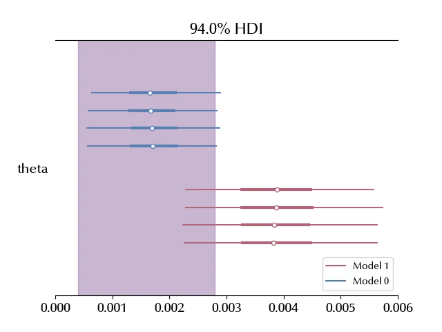
As we can see, there is a substantial preference for model 0. We can better understand this result if we compare our estimate with the frequentist confidence interval, which we recall being \([0.0004, 0.0028]\)
az.plot_forest(traces, figsize=(10, 5), rope=[0.0004, 0.0028])

We can see that the preferred model HDI corresponds with the frequentist CI, while the interval predicted by the second model only partially overlaps with the frequentist CI.
We can also inspect the posterior predictive.
ppc = []
for k, m in enumerate(models):
    with m:
        ppc.append(pm.sample_posterior_predictive(traces[k]))
ppc[0].posterior_predictive['yl'].mean(['chain', 'draw']).values
ppc[1].posterior_predictive['yl'].mean(['chain', 'draw']).values
We recall that the observed value for $y$ was 7, which is much closer to the one provided by the preferred model than to the one provided by Model 1.
Conclusions
In this post we discussed the Bayes factor to choose between different models. In the next post, we will discuss a more powerful method to compare models, namely the Leave One Out cross validation.
%load_ext watermark
%watermark -n -u -v -iv -w -p xarray,pytensor,numpyro,jax,jaxlib
Python implementation: CPython
Python version : 3.12.7
IPython version : 8.24.0
xarray : 2024.9.0
pytensor: 2.25.5
numpyro : 0.15.0
jax : 0.4.28
jaxlib : 0.4.28
pymc : 5.17.0
numpy : 1.26.4
matplotlib: 3.9.2
pandas : 2.2.3
arviz : 0.20.0
Watermark: 2.4.3
