

Gaussian processes
As explained on the stan user guide, gaussian processes, for short GPs, is a powerful tool to perform regression, and its underlying assumption is that the variable $y$ follows a multivariate normal distribution
\[y \sim \mathcal{MvN}(m(x), K(x \vert \theta))\]where $m(\cdot)$ is any function, and it represents the mean, while $K(\cdot \vert \theta)$ is the covariance function, and it is a matrix-valued function.
Since $K(x \vert \theta)$ represents the covariance, it must be a symmetric and positive-defined function of $x\,.$
Different choices of $m$ and $K$ will give different properties to the GP. The two most common choices for $m$ are the constant function and the linear function. The possible choices for the covariance function $K$ are much broader, and here we will discuss some of the most popular choices.
Since the kernel must be a symmetric matrix, its elements must be given by a (scalar) function $k(x, y)\,,$ where we neglect the parameter dependence. A very versatile choice is to assume that the kernel is a function of a scalar combination of $x$ and $y$ (which can be vector-valued), therefore it can depend on $\lVert x-y\rVert^2$ or on $x\cdot y\,.$ In the first case you get a stationary kernel, otherwise you get a polynomial kernel. Stationary kernels are invariant under translation, so their value does not depend on the absolute position on the point, but only on the relative distance from the other points.
In the following, we will restrict our discussion to the one-dimensional case, so we will replace $\lVert x-y \rVert^2$ with $(x-y)^2$ and $x\cdot y$ with $xy\,,$ but it is immediate to recover the general definition.
Notice that, generally, if the dependence on a parameter is multiplicative, then in PyMC the parameter is generally dropped. We will however discuss it since it is useful to understand what role is played by the parameter.
Some common kernel choice
The Rational Quadratic kernel
This kernel is, often, the first choice, due to its nice properties. It has in fact some nice properties one may desire:
- it vanishes as $\lVert x-y \rVert \rightarrow \infty$
- it is a smooth function of $\lVert x-y \rVert^2\,.$
This kernel reads:
\[K(x, y \vert \sigma, \ell) = \sigma^2 \exp{\left( -\frac{(x-y)^2}{2\ell^2} \right)}\]Let us now visualize how does a function distributed according to this kernel behave
import pandas as pd
import pymc as pm
import arviz as az
import numpy as np
from matplotlib import pyplot as plt

xtest = np.linspace(-5, 5, 200)

def kexpquad(x, y, l):
    return np.exp(-(x-y)**2/(2*l**2))

sigma = [0.2, 1, 5]
lng = [0.2, 1, 5]
nplot = 4

fig, ax = plt.subplots(nrows=len(sigma), ncols=len(lng), figsize=(8, 8))
for i, s in enumerate(sigma):
    for j, l in enumerate(lng):
        kf = s**2*np.array([[kexpquad(x, y, l) for x in xtest] for y in xtest])
        for k in range(nplot):
            ax[i][j].plot(xtest, np.random.multivariate_normal(mean=0*xtest, cov=kf))
            ax[i][j].set_title(r"$\sigma=$"+str(s)+r", $\ell=$"+str(l))
fig = plt.gcf()
fig.suptitle(r"$K(x,y)=\sigma^2 \exp\left({-(x-y)^2/(2\ell^2)}\right)$")
fig.tight_layout()
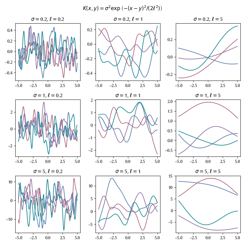
The Rational Quadratic kernel
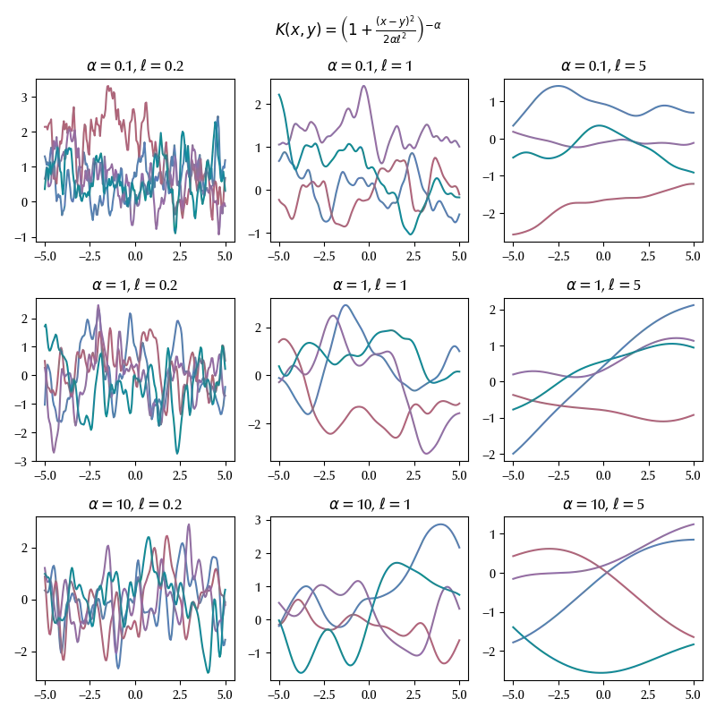
This kernel has the form \(K(x, y) = \left(1+\frac{(x-y)^2}{2\alpha \ell^2}\right)^{-\alpha}\)
is a little bit more versatile than the previous one, since, as explained in this very useful reference, it is equivalent to a linear combination of squared exponential kernels with different $l\,.$ Moreover, as $\alpha \rightarrow \infty\,,$ one recovers the previous kernel.
def kratquad(x, y, a, l):
    return (1+(x-y)**2/(2*a*l**2))**(-a)

alpha = [0.1, 1, 10]
lng = [0.2, 1, 5]
nplot = 4

fig, ax = plt.subplots(nrows=len(alpha), ncols=len(lng), figsize=(8, 8))
for i, a in enumerate(alpha):
    for j, l in enumerate(lng):
        kf = np.array([[kratquad(x, y, a, l) for x in xtest] for y in xtest])
        for k in range(nplot):
            ax[i][j].plot(xtest, np.random.multivariate_normal(mean=0*xtest, cov=kf))
            ax[i][j].set_title(r"$\alpha=$"+str(a)+r", $\ell=$"+str(l))
fig = plt.gcf()
fig.suptitle(r"$K(x,y)=\left(1+\frac{(x-y)^2}{2\alpha \ell^2}\right)^{-\alpha}$")
fig.tight_layout()
Matern kernels
The above kernels are $C^\infty\,,$ and they will ensure $C^\infty\,,$ functions, so they are only appropriate if the underlying data-generation mechanism ensure smoothness. A family of non-smooth kernels is given by the Matérn kernels, which is a family of kernels $K^{Matern}_\nu(x, y, \ell)$ which, in the limit $\nu \rightarrow\infty\,,$ converges to the exponential quadratic kernel.
def kmatern(x, y, p, l):
    if p==0:
        return np.exp(-np.abs(x-y)/l)
    elif p==1:
        return np.exp(-np.sqrt(3)*np.abs(x-y)/l)*(1+np.sqrt(3)*np.abs(x-y)/l)
    elif p==2:
        return np.exp(-np.sqrt(5)*np.abs(x-y)/l)*(1+np.sqrt(5)*np.abs(x-y)/l+5*(x-y)**2/(3*l**2))

pval = [0, 1, 2]
lng = [0.2, 1, 5]
nplot = 4

fig, ax = plt.subplots(nrows=len(pval), ncols=len(lng), figsize=(8, 8))
for i, p in enumerate(pval):
    for j, l in enumerate(lng):
        kf = np.array([[kmatern(x, y, p, l) for x in xtest] for y in xtest])
        for k in range(nplot):
            ax[i][j].plot(xtest, np.random.multivariate_normal(mean=0*xtest, cov=kf))
            ax[i][j].set_title(r"$p=$"+str(p)+r", $\ell=$"+str(l))
fig = plt.gcf()
fig.suptitle(r"$K^{Matern}_{p+1/2}(x,y,\ell)$")
fig.tight_layout()
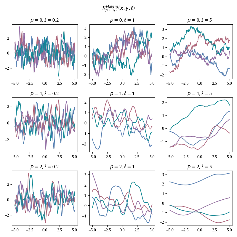
Notice that the $p=0$ kernel is sometimes named exponential or Ornstein-Uhlenbeck kernel, and it defines a Markov process. An GP defined by the exponential kernel is equivalent to an AR(1) process.
The cosine kernel
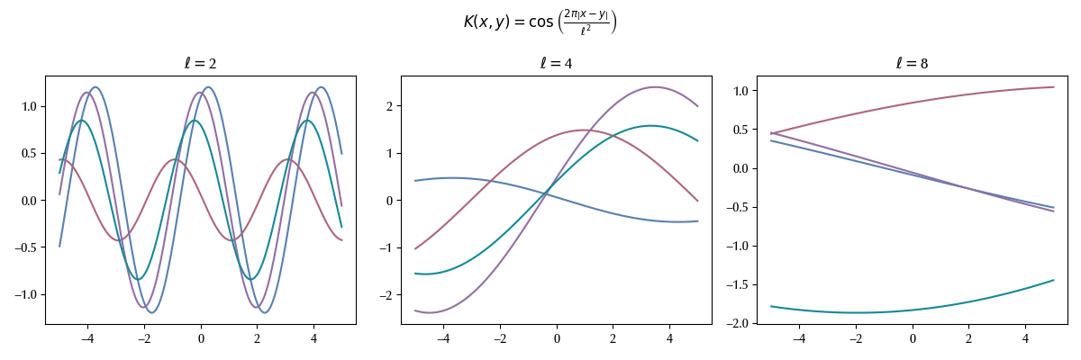
Another property one can encode into GPs is the periodicity. As an example, the cosine kernel gives cosine-shaped functions.
\[K(x, y) = \cos\left( \frac{2 \pi \left|x-y \right|}{\ell^2} \right)\]def kcos(x, y, l):
return np.cos(2.0*np.pi*np.abs(x-y)/l**2)
lng = [2, 4, 8]
nplot = 4
fig, ax = plt.subplots(nrows=1, ncols=len(lng), figsize=(12, 4))
for j, l in enumerate(lng):
kf = np.array([[kcos(x, y, l) for x in xtest] for y in xtest])
for k in range(nplot):
ax[j].plot(xtest, np.random.multivariate_normal(mean=0*xtest, cov=kf))
ax[j].set_title(r"$\ell=$"+str(l))
fig.suptitle(r"$K(x,y)=\cos\left(\frac{2\pi\left| x-y\right|}{\ell^2}\right)$")
fig.tight_layout()
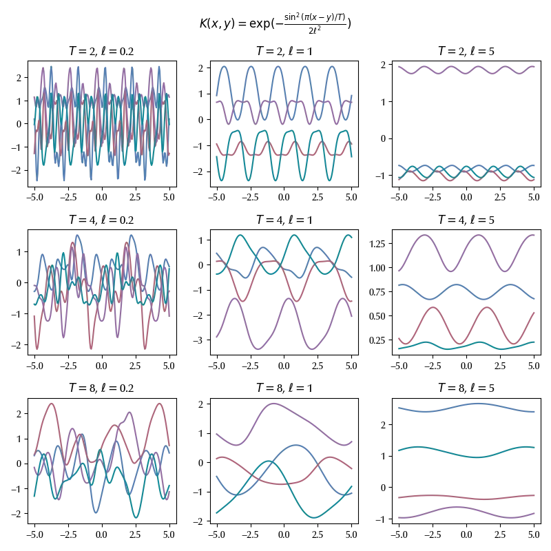
The periodic kernel
Sometimes a cosine is not enough, and you might be interested into a more general form of periodic function. In this case, the periodic kernel might be what you need.
\[K(x, y) = \exp{\left( - \frac{\sin^2{\left(\pi \left(x-y\right)/T\right)}}{2\ell^2} \right)}\]def kperiodic(x, y, T, l):
return np.exp(-np.sin(np.pi*(x-y)/T)**2/(2*l**2))
tval = [2, 4, 8]
lng = [0.2, 1, 5]
nplot = 4
fig, ax = plt.subplots(nrows=len(tval), ncols=len(lng), figsize=(8, 8))
for i, t in enumerate(tval):
for j, l in enumerate(lng):
kf = np.array([[kperiodic(x, y, t, l) for x in xtest] for y in xtest])
for k in range(nplot):
ax[i][j].plot(xtest, np.random.multivariate_normal(mean=0*xtest, cov=kf))
ax[i][j].set_title(r"$T=$"+str(t)+r", $\ell=$"+str(l))
fig.suptitle(r"$K(x,y)=\exp(-\frac{\sin^2(\pi(x-y)/T)}{2\ell^2})$")
fig.tight_layout()
The polynomial kernel
By using GPs one can also perform polynomial regression. The kernel
\[K(x, y) = ((x-c)(y-c))^k\]will sample a monomial of order $k$ with origin $c\,.$
fig, ax = plt.subplots(nrows=3, ncols=len(lng), figsize=(8, 8))

c = [-2, 0, 2]
for i in range(0, 3):
    for j, l in enumerate(c):
        kf = np.array([[((x-l)*(y-l))**i for x in xtest] for y in xtest])
        for k in range(nplot):
            ax[i][j].plot(xtest, np.random.multivariate_normal(mean=0*xtest, cov=kf))
            ax[i][j].set_title(r"$k="+str(i)+", c="+str(l)+"$")
fig = plt.gcf()
fig.suptitle(r"$K(x,y)= ((x-c)(y-c))^k$")
fig.tight_layout()
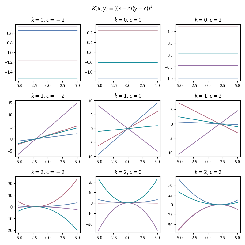
Notice that, if $k=0\,,$ we simply get the constant kernel.
The white noise
Another useful kernel is the white noise. If we take
\[k(x, y) = \sigma^2 I\]where $I$ is the identity matrix, we have that the $n$ dimensional multivariate normal becomes the product of $n$ univariate gaussian distribution, so the points $y_i$ are i.i.d. according to a normal distribution with mean 0 and variance $\sigma\,.$
fig, ax = plt.subplots(nrows=1, ncols=len(lng), figsize=(12, 4))

for j, sig in enumerate(sigma):
    kf = np.eye(len(xtest),len(xtest))*sig**2
    for k in range(nplot):
        ax[j].plot(xtest, np.random.multivariate_normal(mean=0*xtest, cov=kf))
        ax[j].set_title(r"$\sigma=$"+str(sig))
fig = plt.gcf()
fig.suptitle(r"$K(x,y)=\sigma^2 \delta_{ij}$")
fig.tight_layout()
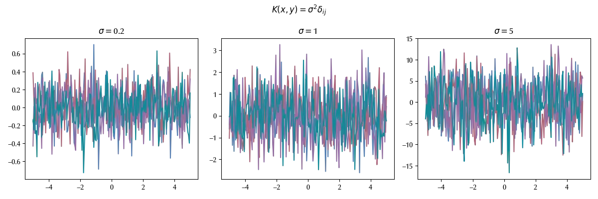
This kernel is usually implemented to encode the fact that the measurements are noisy.
The Brownian motion
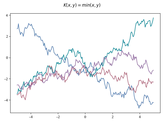
The brownian motion can be considered a GP too, and this process is obtained by using the following kernel:
\[K(x, y) = min(x, y)\]fig = plt.figure()
ax = fig.add_subplot(111)
kf = np.array([[min(x, y) for x in xtest] for y in xtest])
for k in range(nplot):
ax.plot(xtest, np.random.multivariate_normal(mean=0*xtest, cov=kf))
fig.suptitle(r"$K(x,y)=min(x, y)$")
fig.tight_layout()
Building new kernels
We only showed some of the most common kernels, and you could look for new ones by yourself. You can however also build new ones from the previous ones, by only keeping in mind that the covariance matrix must be symmetric and positive-defined. In particular, some possible ways to build new kernels are the following:
- you can take any linear combination $K_1(x, y)+K_2(x, y)$
- you can multiply by any positive scalar $\alpha K(x, y)$
- you can multiply two kernels $K_1(x, y)K_2(x, y)$
- you can replace your variable with any function of it $K(\Phi(x), K(\Phi(y))$
- You can define $\Phi(x) K(x, y) \Phi(y)$ for any positive $\Phi(x)\,.$
- You can take the convolution of a kernel with any positive function $\int dx dy K(x, y)f(x-x_0)f(y-y_0)$
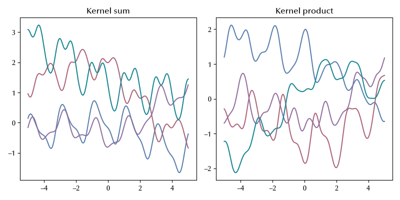
As an example, if you take as kernel the superposition of a squared exponential kernel and a periodic kernel, you will get a periodic signal superimposed to a squared exponential GP. On the other hand, if you multiply them, you will get a periodic kernel with varying amplitude.
fig = plt.figure(figsize=(8, 4))
ax = fig.add_subplot(121)
kf = np.array([[kperiodic(x, y, 2, 1)+kexpquad(x, y, 3) for x in xtest] for y in xtest])
for k in range(nplot):
    ax.plot(xtest, np.random.multivariate_normal(mean=0*xtest, cov=kf))
# fig.suptitle(r"$K(x,y)=min(x, y)$")

ax1 = fig.add_subplot(122)
kf = np.array([[kperiodic(x, y, 2, 1)*kexpquad(x, y, 3) for x in xtest] for y in xtest])
for k in range(nplot):
    ax1.plot(xtest, np.random.multivariate_normal(mean=0*xtest, cov=kf))
fig.tight_layout()
Conclusions
I home I managed to convince you that GPs can be extremely powerful to add flexibility and encod desired properties into your models, and in the next post we will discuss some practical application.