Gaussian processes regression

In the last post, we introduced GPs. In this post we will see how to use them in order to perform regression in a non-parametric fashion. We will use the Nile dataset, which contains the Nile flow, expressed in $10^8 m^3$ measurements from 1871 to 1970.

Implementation

Let us first of all download the dataset.

import numpy as np
import pandas as pd
import pymc as pm
import pymc_experimental.distributions as pmx
import seaborn as sns
import arviz as az
from matplotlib import pyplot as plt

rng = np.random.default_rng(42)

df = pd.read_csv("https://raw.githubusercontent.com/vincentarelbundock/Rdatasets/master/csv/datasets/Nile.csv")

df['time'] = df['time'].astype(int)

sns.scatterplot(df, x='time', y='value')
fig = plt.gcf()
fig.tight_layout()

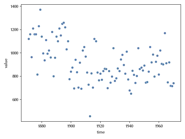
The data seems almost stationary, except from a small discontinuity just before 1900, and it also shows some auto-correlation, as they don’t look i.i.d. at all, and it looks like there is no obvious periodicity.

The dataset contains 100 points, and we will use the first 85 to fit our model, while the last 15 points will be used to assess the performances of our model in predicting the future flow.

n = 85
df_train = df.iloc[:n]
df_test = df.iloc[n:]

x_train = (df_train['time']-df_train['time'].iloc[n//2])
x_test = (df_test['time']-df_train['time'].iloc[n//2])
x_test /= np.max(x_train)
x_train /= np.max(x_train)

We normalized the regression variables so that it is bounded between -1 and 1. It will be convenient to have it normalized in this way, as it will simplify some parameter estimate.

One of the main issues of GPs is given by their performances. However, when you are working with local kernels, by truncating the Fourier series expansion of the Kernel, you can obtain what is usually named as “Hilbert Space GPs”, and this allows a faster implementation of the GPs. This is not possible for all the kernels, as the Fourier series must exist.

with pm.Model() as model:
    lam = pm.HalfNormal('lam', 0.15)
    tau = pm.Exponential('tau', 2)
    rho = pm.Normal('rho', 1)
    gp = pm.gp.HSGP(m=[25], L=[1.2], mean_func=pm.gp.mean.Constant(rho),cov_func=tau*pm.gp.cov.ExpQuad(1, lam))
    mu = gp.prior('mu', X=x_train.values.reshape((-1, 1)))
    sigma = pm.HalfNormal('sigma', 1)
    y = pm.Normal('y', mu=mu, sigma=sigma, observed=df_train['value']/1000)

We used a squared exponential kernel, where we assume that the GP fluctuations are of the order of 0.5. The parameter L must be chosen so that all the points are included into $[-L, L]\,,$ and this is why we normalized the regression variable as above. We assumed that the mean of the GP has absolute value less than 2, and this seems reasonable given the dataset. We only kept 25 terms in the Fourier expansions, and later we will see how to verify if we did a meaningful choice.

with model:
    idata = pm.sample(nuts_sampler='numpyro',
                     draws=5000, tune=5000, random_seed=rng, target_accept=0.95)

az.plot_trace(idata)
fig = plt.gcf()
fig.tight_layout()

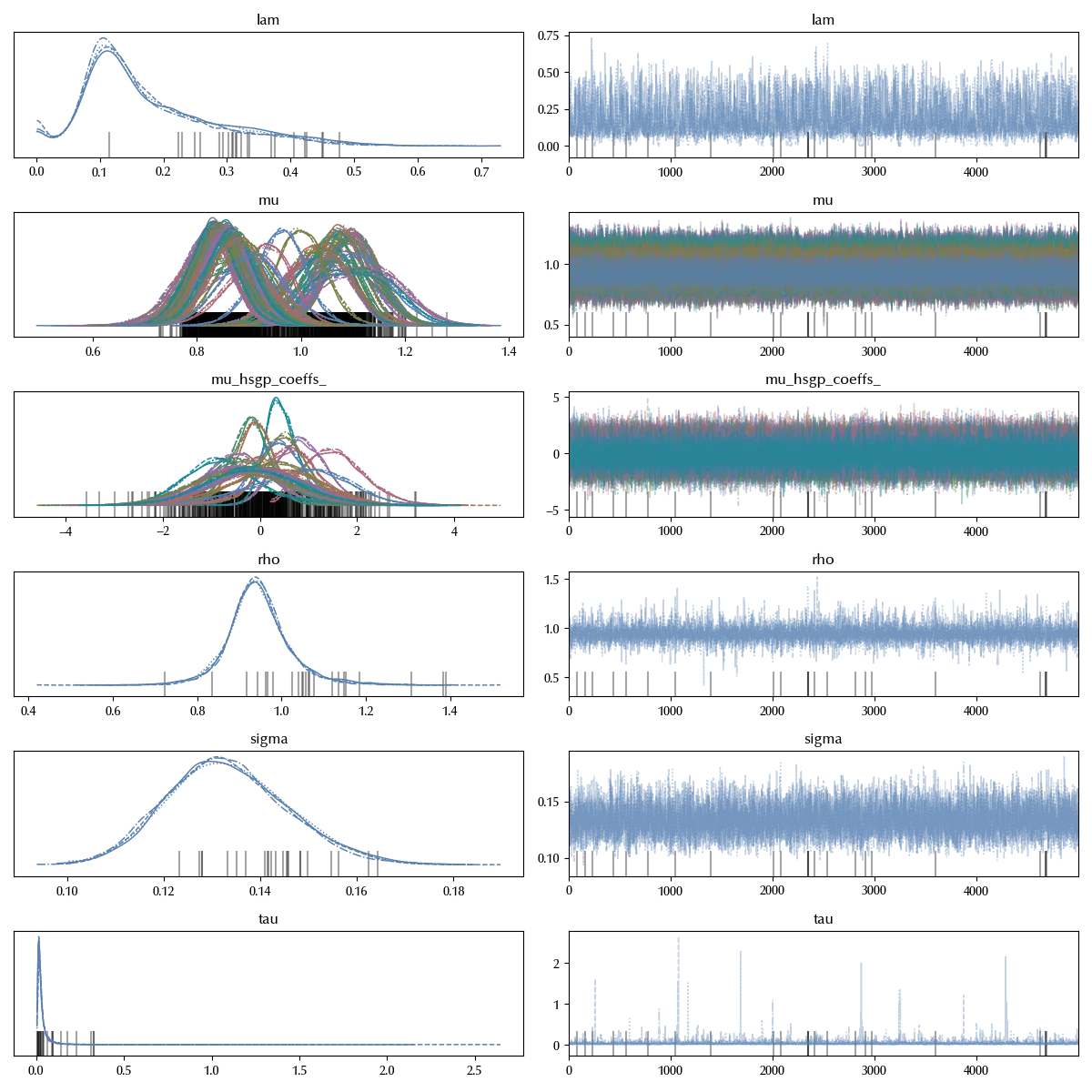
It looks like there are few divergences, but this is not a big issue, as their number is very small and the traces don’t show relevant issues.

Since we truncated the Fourier series, we would like that the last few coefficients of the series expansion are close to 0, otherwise we would have an indications that the series has been truncated too early.

az.plot_forest(idata, var_names=['mu_hsgp_coeffs_'])
fig = plt.gcf()
fig.tight_layout()

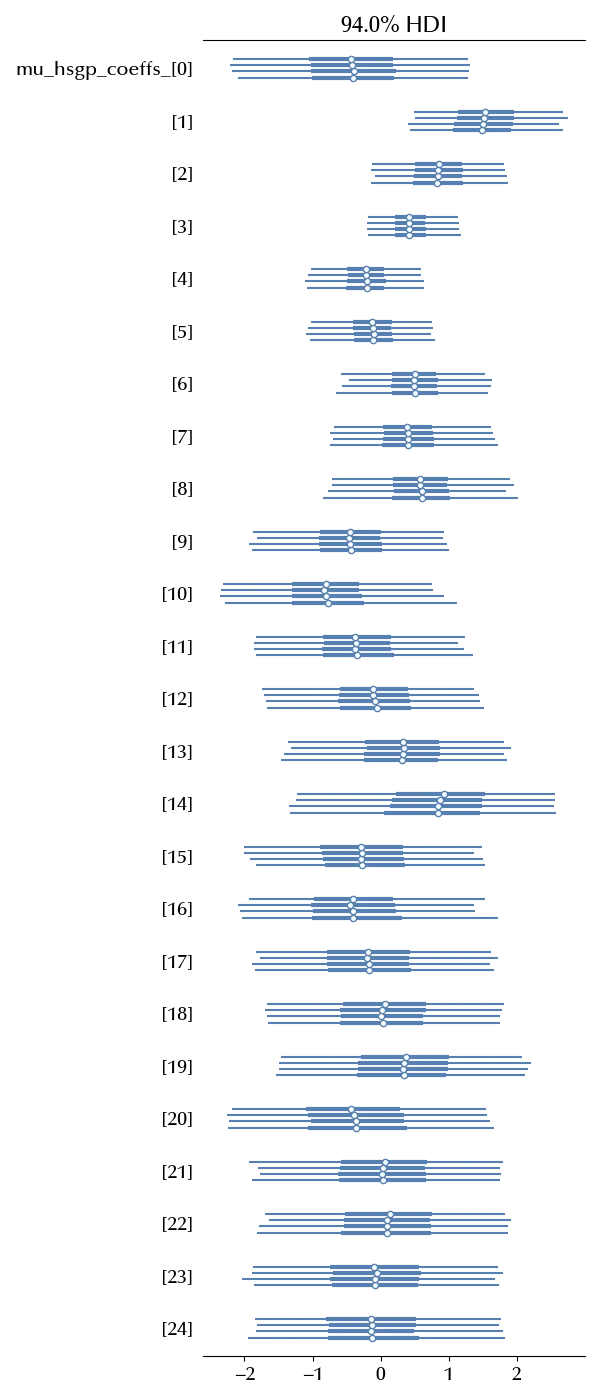
The coefficients are almost zero starting from $i = 20\,,$ so the truncation seems ok. We can now inspect the posterior predictive.

with model:
    idata.extend(pm.sample_posterior_predictive(idata))

fig = plt.figure()
ax = fig.add_subplot(111)
ax.fill_between(df_train['time'], 1000*idata.posterior_predictive['y'].quantile(q=0.03, dim=('draw', 'chain')),
               1000*idata.posterior_predictive['y'].quantile(q=0.97, dim=('draw', 'chain')),
               color='lightgray', alpha=0.8)
ax.plot(df_train['time'], 1000*idata.posterior_predictive['y'].mean(dim=('draw', 'chain')))
sns.scatterplot(df, x='time', y='value', ax=ax)
ax.set_xlim([df_train['time'].iloc[0], df_train['time'].iloc[-1]])

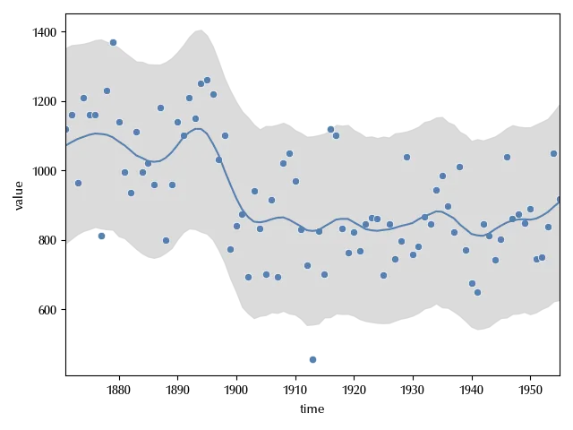
In the “train” region we can reproduce with quite a high accuracy the observed data, and there is no obvious sign of overfitting issues. We can now use the remaining years to verify the performances of our model when predicting new data.

with model:
    mu_pred = gp.conditional('mu_pred', Xnew=x_test.values.reshape((-1, 1)))
    y_pred = pm.Normal('y_pred', mu=mu_pred, sigma=sigma)

with model:
    ppc = pm.sample_posterior_predictive(idata, var_names=['mu_pred', 'y_pred'])

ypred = np.concatenate([idata.posterior_predictive['y'].values.reshape((20000, 85)),
ppc.posterior_predictive['y_pred'].values.reshape((20000, 15))], axis=1)

fig = plt.figure()
ax = fig.add_subplot(111)
ax.fill_between(df['time'], 1000*np.quantile(ypred, q=0.03, axis=0),
               1000*np.quantile(ypred,q=0.97, axis=0),
               color='lightgray', alpha=0.8)
ax.plot(df['time'], 1000*np.mean(ypred, axis=0))

ax.axvline(x=df_test['time'].iloc[0], ls=':', color='k')
sns.scatterplot(df, x='time', y='value', ax=ax)
ax.set_xlim([df['time'].iloc[0], df['time'].iloc[-1]])

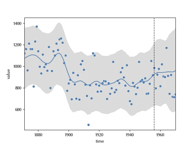
The credible interval seems large enough to accommodate all the observed data, and it does not explode. We can be therefore quite confident into the performances of our model.

Conclusions

We used GPs to perform regression over the Nile dataset. We introduced HSGPs, and we briefly explained how to use them and how to assess the goodness of the approximation.

Implementation

Conclusions

Suggested readings