

Splines
GPs are very flexible, but their implementation becomes tricky when the number of points grows too much. If you are experiencing this kind of issue when performing regression, a possible alternative is to use splines.
Splines are piecewise-defined functions, appropriately matched in order to ensure smoothness to the resulting function. There are many spline families, and we will focus on B-splines, as they are very easy to implement and numerically very stable (while this might not be true for other kind of splines such as polynomial splines). You will find more on this topic on the PyMC gallery, where the PyMC team used Patsy to implement the splines. We will instead do it from scratch, as it might be instructive to see how to do so.
Given a set of $m+1$ points named knots $t_0,t_1,\dots,t_m\,,$ B-splines are recursively defined:
\[B_{i,0}(t) = \begin{cases} 1 & t_i \leq t < t_{i+1} \\ 0 & otherwise \\ \end{cases}\]One can then define higher order splines as
\[B_{i,p}(t) = \frac{t-t_i}{t_{i+p}-t_i} B_{i,p-1}(t) + \frac{t_{i+p+1}-t}{t_{i+p+1}-t_{i+1}} B_{i+1,p-1}(t)\]We can therefore search for our target function by expanding it in terms of B-splines of order $p$
\[f(t) = \sum_i \alpha_i B_{i, p}(t)\]The FEV dataset
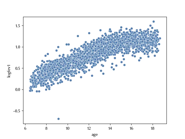
We will use B-spline to perform non-parametric regression on the “Six Cities Study of Air Pollution and Health” from “Applied Longitudinal Analysis”, which can be found on the book webpage. This dataset is a subsample of the measures of the Forced Expiratory Volume (FEV), expressed in liters, for 300 girls living in the Topeka city, with age ranging from 6 to 19. Our aim will be to determine the relation between the age and the FEV (logarithm).
import pandas as pd
import numpy as np
from matplotlib import pyplot as plt
import seaborn as sns
import pymc as pm
import arviz as az

df = pd.read_stata('data/fev1.dta')

rng = np.random.default_rng(42)

df['id'] = df['id'].astype(int)

df.head()
| id | ht | age | baseht | baseage | logfev1 | |
|---|---|---|---|---|---|---|
| 0 | 1 | 1.2 | 9.3415 | 1.2 | 9.3415 | 0.21511 |
| 1 | 1 | 1.28 | 10.3929 | 1.2 | 9.3415 | 0.37156 |
| 2 | 1 | 1.33 | 11.4524 | 1.2 | 9.3415 | 0.48858 |
| 3 | 1 | 1.42 | 12.46 | 1.2 | 9.3415 | 0.75142 |
| 4 | 1 | 1.48 | 13.4182 | 1.2 | 9.3415 | 0.83291 |
sns.scatterplot(df, x='age', y='logfev1')
Let us now implement the function to compute the splines
def bspline(t: np.array, x:np.array, i:int, p:int) -> float:
    """
    Returns a B-spline, defined as https://en.wikipedia.org/wiki/B-spline.

    Parameters:
    -----------
    t: np.array
    x: np.array
    i: int
    p: int

    Returns:
    np.array

    Raises:
    ------
    ValueError
       if i is not an integer between 0 and len(x)-p-1 (both included)
    """
    if i>=0 and i<len(x)-p-1:
        if p==0:
            return np.heaviside(t-x[i], 1)*np.heaviside(x[i+1]-t, 0)
        else:
            fac0 = (t-x[i])/(x[i+p]-x[i])
            fac1 = (x[i+p+1]-t)/(x[i+p+1]-x[i+1])
            return (fac0*bspline(t, x, i, p-1)+fac1*bspline(t, x, i+1, p-1))
    else:
        raise ValueError(f'Got i={i}, i must be an integer between 0 and len(x)-p-1={len(x)-p-1}')
Let us now take a look at the splines.
x_plot = np.arange(5, 20, 0.1)
x_fit = np.linspace(5, 20, 15)

basis_plot_0 = np.array([bspline(x_plot, x_fit, i, 0) for i in range(len(x_fit)-1)])
basis_plot_1 = np.array([bspline(x_plot, x_fit, i, 1) for i in range(len(x_fit)-2)])
basis_plot_2 = np.array([bspline(x_plot, x_fit, i, 2) for i in range(len(x_fit)-3)])

fig, ax = plt.subplots(nrows=3)
for elem in basis_plot_0:
    ax[0].plot(x_plot, elem)
    ax[0].set_title(r"$p=0$")
for elem in basis_plot_1:
    ax[1].plot(x_plot, elem)
    ax[1].set_title(r"$p=1$")
for elem in basis_plot_2:
    ax[2].plot(x_plot, elem)
    ax[2].set_title(r"$p=2$")
fig.tight_layout()
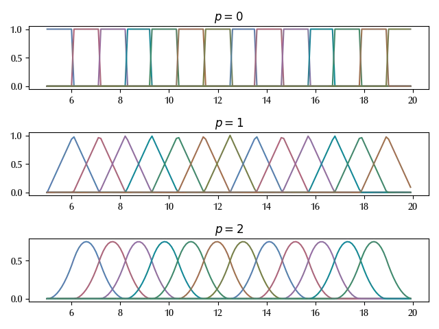
As you can see, a B-spline of order $p$ can be differentiated $p-1$ times. We will only assume the existence of the first derivative, so we will use second-order splines. The knots defined above look dense enough, we will therefore use them.
p_fit = 2

splines_dim = len(x_fit)-p_fit-1

basis = np.array([bspline(df['age'].values, x_fit, i, p_fit) for i in range(splines_dim)])
We pre-computed the splines in order not to waste computational time, and we are now ready to implement our model. We will assume a linear plus spline model in order to easily encode the trend which is present in for younger girls.
with pm.Model() as spline_model:
    alpha = pm.Normal('alpha', mu=0, sigma=1)
    beta = pm.Normal('beta', mu=0, sigma=1)
    w = pm.Normal('w', mu=0, sigma=20, shape=(splines_dim))
    sigma = pm.Exponential('sigma', lam=1)
    mu = alpha + beta*df['age'] + pm.math.dot(w, basis)
    yhat = pm.Normal('yhat', mu=mu, sigma=sigma, observed=df['logfev1'])

with spline_model:
    idata_spline = pm.sample(nuts_sampler='numpyro', draws=5000, target_accept=0.9, random_seed=rng)

az.plot_trace(idata_spline)
fig = plt.gcf()
fig.tight_layout()
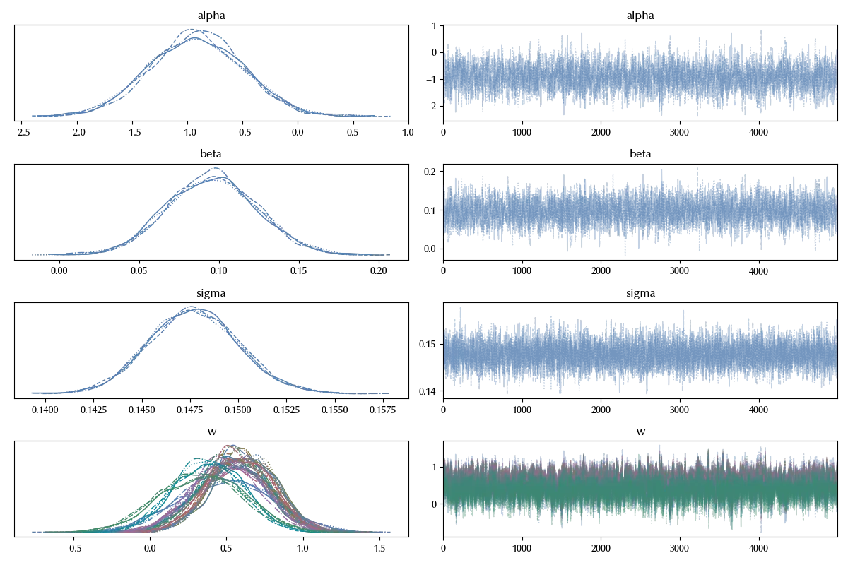
The trace looks fine, let us now inspect the predicted FEV
with spline_model:
    mu_pred = pm.Deterministic('mu_pred', alpha + beta*x_plot + pm.math.dot(w, basis_plot_2))
    yhat_pred = pm.Normal('yhat_pred', mu=mu_pred, sigma=sigma)

with spline_model:
    ppc_spline = pm.sample_posterior_predictive(idata_spline, var_names=['yhat_pred', 'mu_pred'])

fig = plt.figure()
ax = fig.add_subplot(111)
ax.plot(x_plot,
ppc_spline.posterior_predictive['yhat_pred'].mean(dim=['draw', 'chain']))
ax.fill_between(x_plot,
ppc_spline.posterior_predictive['yhat_pred'].quantile(q=0.025, dim=['draw', 'chain']),
ppc_spline.posterior_predictive['yhat_pred'].quantile(q=0.975, dim=['draw', 'chain']),
                color='lightgray', alpha=0.8
               )
ax.scatter(df['age'], df['logfev1'], color='gray', alpha=0.8)
ax.set_xlim([x_plot[0], x_plot[-1]])
fig.tight_layout()
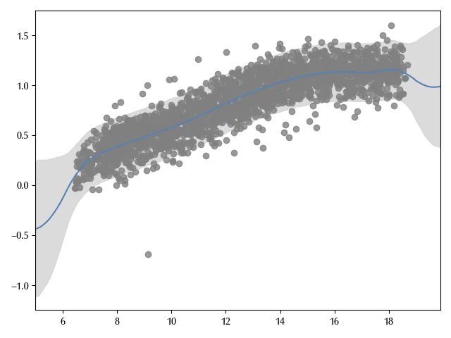
As we can see, our model both reproduces the linear growth and the saturation of the FEV which starts at about 15.
As a general warning, you should always keep in mind that b-splines vanish outside from their basis domain, so if you use them to catch some relevant behavior which is needed to appropriately describe the desired behavior outside, you might have a bad surprise when you try and generalize.
Conclusions
We introduced the concept of spline, and we have seen how to implement B-splines in a PyMC model. We used this model to fit the “Six Cities Study of Air Pollution and Health” dataset.
%load_ext watermark
%watermark -n -u -v -iv -w -p xarray,numpyro,jax,jaxlib
Python implementation: CPython
Python version : 3.12.4
IPython version : 8.24.0
xarray : 2024.5.0
numpyro: 0.15.0
jax : 0.4.28
jaxlib : 0.4.28
numpy : 1.26.4
pymc : 5.15.0
arviz : 0.18.0
matplotlib: 3.9.0
seaborn : 0.13.2
pandas : 2.2.2
Watermark: 2.4.3