Bayesian Additive Regression Trees

A Bayesian Additive Regression Tree (BART) is a black box Bayesian method proposed in 2010 to approximate functions, and it can be useful when you need to interpolate your data, but it is hard to figure out a transparent way to do so. BART can be considered as the bayesian counterpart of a random forest regression, where we assign a prior to each regression tree.

More specifically, BART assumes

\[Y \sim f(X) + \varepsilon\]

where $\varepsilon$ is normally distributed, and

\[f(X) = \sum_i g_i(X, T_i, M_i)\]

Here $T_i$ represents a binary tree, and $M_i$ the set of means associated to $T_i$ In practice, a binary tree can be seen as a set of if-else, and an example is

\[g_0 = \begin{cases} X < c_1 & \mu_1 \\ X \geq c_1 & \begin{cases} X < c_2 & \mu_2 \\ X \geq c_2 & \mu_3 \\ \end{cases} \\ \end{cases}\]

BART is a Bayesian method because both $T_i$ and $M_i$ are regularized by using priors.

BART is

Bayesian
Additive
binary Regression Trees

Regression trees are powerful tools to capture interactions, as they are a collection of if-else statements. Each tree tries and initially reproduce the typical value, while the interaction terms are captured by the periferic branches. A single tree can however only capture stepwise behaviors, and this is why we don't only consider a single tree, but we rather construct a sum of trees. This improves the capacity to capture linear behaviors. We finally attach a prior to each node and to each tree, by making more likely small trees, with only few branches, with small averages. A proper prior choice together with the initial normalization of the variables balances flexibility with the possibility to overfit the data. In PyMC, the default number of trees $m$ is taken to be 50, but PSIS-LOO can be effectively used to tune this parameter. Notice that the construction of a binary tree includes the number of nodes as a parameter, this is the reason why BART cannot be sampled with HMC, but an ad-hoc Metropolis-Hastings sampler is implemented.

For a more in-depth discussion about BARTs, you can take a look at this preprint or at the PyMC-BART homepage.

The diamond dataset

We will use BART to fit the diamond dataset, which is dataset proposed in this article to show some of the main issues you will have to deal with when fitting real-World datasets. I strongly encourage you to read this article, as it is a very instructive example of some of the issues most data scientist faced when working to real problems.

import seaborn as sns
import pandas as pd
from matplotlib import pyplot as plt
import numpy as np
import pymc as pm
import arviz as az
import arviz_plots as azp
import pymc_bart as pmb

df = pd.read_csv('https://vincentarelbundock.github.io/Rdatasets/csv/Ecdat/Diamond.csv')

rng = sum(map(ord, 'BART'))

df.head()

	rownames	carat	colour	clarity	certification	price
0	1	0.3	D	VS2	GIA	1302
1	2	0.3	E	VS1	GIA	1510
2	3	0.3	G	VVS1	GIA	1510
3	4	0.3	G	VS1	GIA	1260
4	5	0.31	D	VS1	GIA	1641

sns.scatterplot(df, x='carat', y='price')

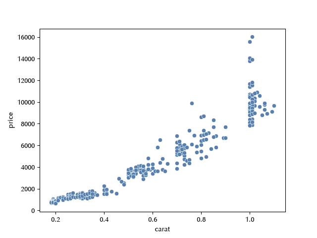
As we can see, it appears that the relation between carat number and price is non-linear, and the price also looks heteroscedastic with respect to the price. We will use BART both the mean and the variance of a normal distribution. First of all, let us convert the categorical variables into a meaningful way:

X = pd.concat([pd.get_dummies(df['colour']).astype(int),
               pd.get_dummies(df['clarity']).astype(int),
               pd.get_dummies(df['certification']).astype(int),
               df['carat']], axis=1)

yobs = df['price']/1000

We also scaled the observations in order to simplify the work to the algorithms. We can now implement the model as follows

with pm.Model(coords={'obs': X.index, 'cols': X.columns}) as model_carat:
    Xv = pm.Data('Xv', X)
    w = pmb.BART("w", X=Xv, Y=np.log(yobs), m=20, shape=(2, len(yobs)))
    y = pm.Normal("y", mu=pm.math.exp(w[0]), sigma=pm.math.exp(w[1]), observed=yobs)

with model_carat:
    idata = pm.sample(draws=3000, tune=3000, random_seed=rng)

az.plot_trace(idata)
fig = plt.gcf()
fig.tight_layout()

The trace of the BART model

It is really hard to verify if there is any numerical issue with the sampling. It is in fact generally recommended to only use it for the non-BART part of the model, which is absent here. PyMC-BART comes in fact with its own routines for the convergence assessment.

azp.plot_convergence_dist(idata)
fig = plt.gcf()
fig.tight_layout()

The trace of the BART model
using PyMC-BART

The curves in the left-hand plot are entirely above the dashed line, while the ones in the right-hand figure are mostly below the corresponding dashed line, and this tells us that our computation can be considered as reliable.

Notice that we haven’t used numpyro as usual, as we cannot use it together with PyMC-BART. This is however not a problem, since PyMC is fast enough.

We can now inspect the posterior predictive distribution

posterior_mean = idata.posterior["w"].mean(dim=("chain", "draw"))[0]

w_hdi = az.hdi(ary=idata, group="posterior", var_names=["w"], hdi_prob=0.5)

with model_carat:
    ppc = pm.sample_posterior_predictive(idata)

pps = az.extract(
    ppc, group="posterior_predictive", var_names=["y"]
).T

idx = np.argsort(Xv[:, -1])

fig, ax = plt.subplots()

az.plot_hdi(
    x=df['carat'],
    y=pps.values,
    ax=ax,
    hdi_prob=0.90,
    fill_kwargs={"alpha": 0.3, "label": r"Observations $90\%$ HDI"},
)

ax.scatter(
    x=df['carat'],
    y=np.exp(posterior_mean.values),
    marker='x'
)

ax.scatter(df['carat'], yobs)
# ax.plot(df["youtube"], df["sales"], "o", c="C0", label="Raw Data")
ax.legend(loc="upper left")

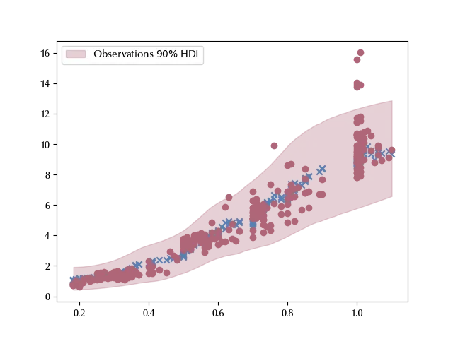
Except from few extreme cases, our model seems appropriate to describe the observed price. We can also assess the variable importance.

vi_results = pmb.compute_variable_importance(idata, w, X)

fig, ax = plt.subplots()
pmb.plot_variable_importance(vi_results, ax=ax)
tksl = ax.get_xticklabels()
ax.set_xticklabels(tksl, rotation=45)
ax.set_ylim([0.8, 1])
fig.tight_layout()

The variable importance plot

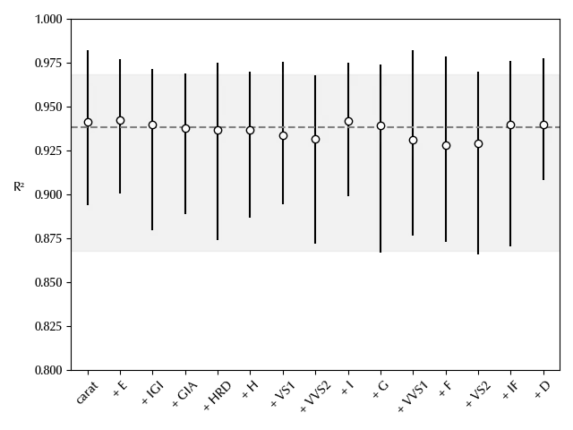
We can finally visualize the marginal dependence of the model on the single variables

pmb.plot_pdp(w, X, np.log(yobs), figsize=(9, 11), grid=(8, 4),
            var_discrete=list(range(14)))
fig = plt.gcf()
fig.tight_layout()

The marginal dependence plot

Conclusions

We introduced BARTs, and we showed how to use them in PyMC by applying them to the diamonds dataset.

The diamond dataset

Conclusions

Suggested readings