Dirichlet Process Mixture Models

In a previous post we discussed parametric mixture models, which are mixture models where the number of components are fixed. These models are more flexible than the respective one-component model, but there are situations in which this flexibility is not enough, since one does not know in advance the number of components to take.

One could naively try and assume a large number of components in a mixture model, unfortunately this is not a good idea, as the behavior of the Dirichlet distribution is ill-defined as the number of components $K$ diverges.

Dirichlet Processes Mixture Models, or DPMMs, are the appropriate way to generalize mixture models, as the limit $K \rightarrow \infty$ is well-defined. Here we will only give an intuitive justification to DPs, and the interested reader will find a more formal discussion in the bibliography. Rather than assuming

\[\pi \vert \alpha \sim \mathcal{Dir}(\alpha,\dots, \alpha)\]

one simply has to assume

\[\pi \vert \alpha \sim \mathcal{Dir}(\alpha/K,\dots, \alpha/K)\,.\]

While this behavior is well-defined from a theoretical point of view, it is not a good idea to implement the above formula in order to sample the prior distribution, since this method is prone to numerical errors as $K$ grows. The most reliable way, at the moment, to sample from a DP, is to use the stick breaking process

\[\begin{align*} \theta_1,\dots,\theta_K \sim & B(1, \alpha) \\ \pi_1 = & \theta_1 \\ \pi_i = & \theta_i \prod_{j<i} (1-\theta_j) \end{align*}\]

DPMMs have been extensively applied to many fields, and they are currently very popular in the text classification, as the number of topics is generally not previously known.

Application to the In-Home Geriatric Assessment dataset

In this section we will apply DPMMs to the IHGA dataset, as already done in this study. In the randomized clinical trial, a set of 572 elderly people has been randomly assigned to one of two groups. The control group, made of 287 units, received the standard health care, while the remaining units received the standard health care plus an experimental preventive treatment. The number of hospitalizations for the individuals has been therefore been monitored for two years.

Hospitalizations	0	1	2	3	4	5	6	7
Control	138	77	46	12	8	4	0	2
Treatment	147	83	37	13	3	1	1	0

As in the cited document, we will use a DPMM, but we will use an uninformative Gamma prior for the average number of hospitalizations, adapting the model proposed in this PyMC example to our needs. We will assume two identical models for the test group and for the control one, and we will then compare the number of hospitalizations averaged over the sample in order to assess the effectiveness of the treatment.

import numpy as np
import pandas as pd
import seaborn as sns
from matplotlib import pyplot as plt
import pymc as pm
import arviz as az
import statsmodels as sm

rng = np.random.default_rng(42)

n_control = [138, 77, 46, 12, 8, 4, 0, 2]

nhosp_control = sum([[i]*elem for i, elem in enumerate(n_control)],[])

n_test = [147, 83, 37, 13, 3, 1, 1, 0]

nhosp_test = sum([[i]*elem for i, elem in enumerate(n_test)],[])

K = 10

with pm.Model() as model_c:
    alpha_c = pm.Gamma("alpha_c", 1.0, 1.0)
    w_c = pm.StickBreakingWeights('w_c', alpha=alpha_c, K=K-1)
    lam_c = pm.Gamma("lam_c", 1/10, 1/10, shape=(K))
    y_c = pm.Mixture(
        "y_c", w_c, pm.Poisson.dist(lam_c), observed=nhosp_control)

with pm.Model() as model_t:
    alpha_t = pm.Gamma("alpha_t", 1.0, 1.0)
    w_t = pm.StickBreakingWeights('w_t', alpha=alpha_t, K=K-1)
    lam_t = pm.Gamma("lam_t", 1/10, 1/10, shape=(K))
    y_t = pm.Mixture(
        "y_t", w_t, pm.Poisson.dist(lam_t), observed=nhosp_test
    )

with model_c:
    idata_c = pm.sample(nuts_sampler='numpyro',
                        draws=2000, tune=2000, random_seed=rng, target_accept=0.9)

with model_t:
    idata_t = pm.sample(nuts_sampler='numpyro',
                        draws=2000, tune=2000, random_seed=rng, target_accept=0.9)

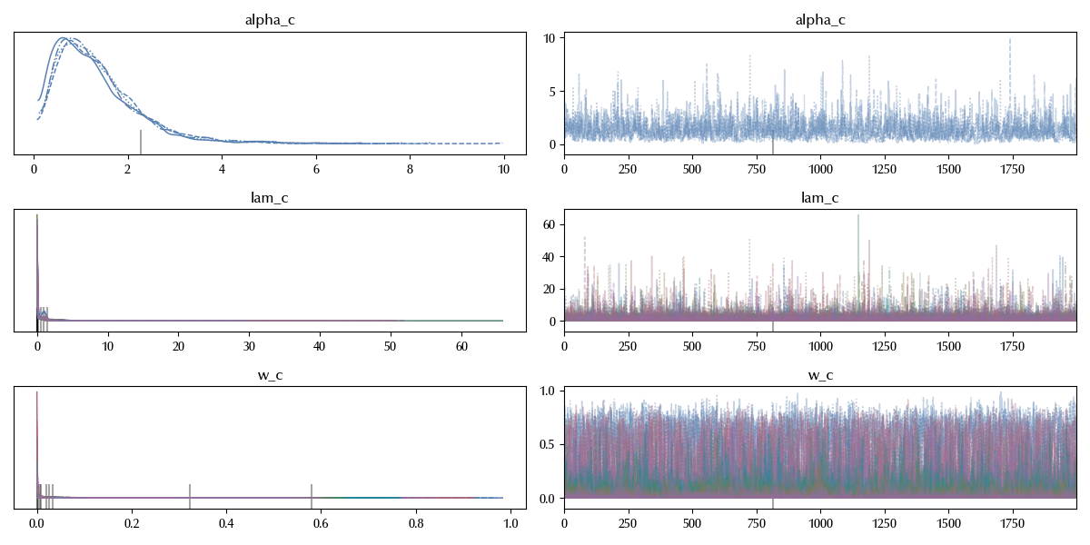
We can now inspect the traces of our models.

az.plot_trace(idata_c)
fig = plt.gcf()
fig.tight_layout()

az.plot_trace(idata_t)
fig = plt.gcf()
fig.tight_layout()

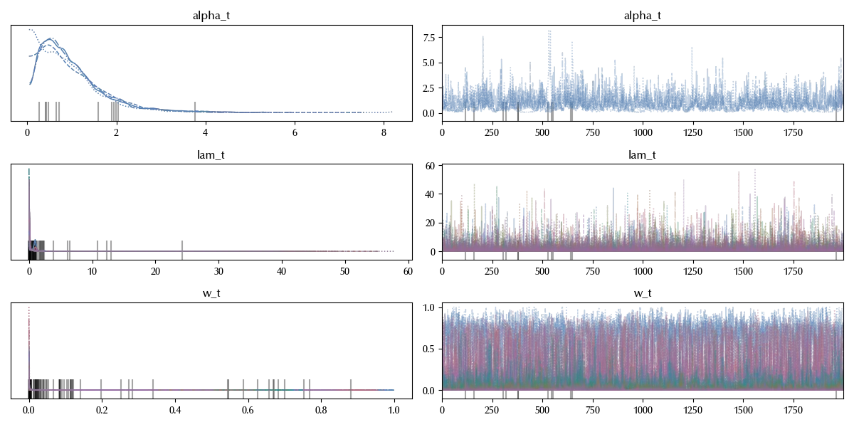
There are few divergences, but this is not a big issue. This is quite normal, as sampling from a DP is numerically demanding due to the large correlations of the weights.

We can now verify if our models can reproduce the observed data

with model_c:
    idata_c.extend(pm.sample_posterior_predictive(idata_c))

with model_t:
    idata_t.extend(pm.sample_posterior_predictive(idata_t))

fig = plt.figure()
ax = fig.add_subplot(211)
bins = np.arange(50)
for elem in az.extract(idata_t, group='posterior_predictive', var_names=['y_t'], num_samples=1000).T:
    ax.hist(elem, histtype='step', color='lightgray', alpha=0.8,
           bins=bins, density=True)
ax.hist(nhosp_test, histtype='step',bins=bins, color='k', density=True)
ax.set_xlim([bins[0], bins[-1]])
ax.set_title('Test group')

ax1 = fig.add_subplot(212)
for elem in az.extract(idata_c, group='posterior_predictive', var_names=['y_c'], num_samples=1000).T:
    ax1.hist(elem, histtype='step', color='lightgray', alpha=0.8,
           bins=bins, density=True)
ax1.hist(nhosp_control, histtype='step',bins=bins, color='k', density=True)
ax1.set_xlim([bins[0], bins[-1]])
ax1.set_title('Control group')
fig.tight_layout()

The PPC of our models

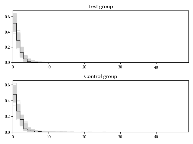
The agreement is more than satisfactory, but it is hard to assess which model is better by simply looking at the above figures. We can however easily compare the distributions of the number of hospitalizations averaged over the individuals.

mu_t = idata_t.posterior_predictive['y_t'].mean(dim=('y_t_dim_2')).values.reshape(-1)
mu_c = idata_c.posterior_predictive['y_c'].mean(dim=('y_c_dim_2')).values.reshape(-1)

fig = plt.figure()
ax = fig.add_subplot(111)
az.plot_posterior(mu_t/mu_c, ax=ax)
ax.set_title(r'$\mu_t/\mu_c$')

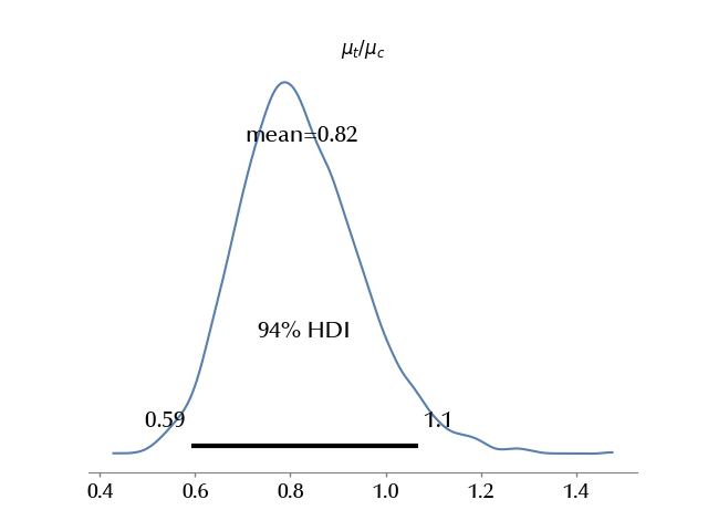
The ratio of the average number of hospitalizations

We are therefore quite confident in concluding that the treatment group has an average number of hospitalizations than the control group.

Conclusions

We have seen how DPMMs generalize Dirichlet Mixtures to an unknown number of components, and we have seen an application of this kind of model to the IHGA dataset.

Application to the In-Home Geriatric Assessment dataset

Conclusions

Suggested readings