Differential equations

Few days ago I started reading Gause’s book The Struggle for Existence: A Classic of Mathematical Biology and Ecology. It’s a beautiful textbook on mathematical ecology, and even if its almost 100 years old and some concepts might be outdated, I think it contains many useful examples which explain how science works, or at least should work.

The textbook contains many applications of the Lotka-Volterra model to systems with competing resources. There are many beautiful figures, and all the data has been exported in this amazing GitHub repo ¹.

I therefore decided to look at the Lotka-Volterra model, and I started with the simplest example: the one specie case. This model describes the number of individuals of a species. When there are many resources, the individuals reproduce themselves, and the model assumes that

\[\frac{dN(t)}{dt} \approx \lambda N\]

The solution of the above differential equation is

\[N(t) = N_0 e^{\lambda t}\]

and this diverges as $t$ grows, but since the number of units cannot however grow indefinitely, as there is a limited amount of space and resources. We therefore define the maximum number of units as $K$, and we can modify the above differential equation into the following one

\[\frac{dN(t)}{dt} = \lambda N (1-\frac{N}{K})\]

If $N \ll K$ we recover back the exponential growth, but if $N$ approaches $K$ then we have $\frac{dN(t)}{dt} \rightarrow 0\,,$ as required.

The above differential equation is known as the logistic differential equation, and you already encountered its solution when we discussed the GLM model, but since it’s better to start with the simplest model as possible, I first tried to implement this model before moving to the version of the equations with more than one specie.

When you implement a numerical algorithm there are many things which might go wrong, as you might have missed a factor 2, or your choice for some parameter might have introduced some instability. It is therefore a very good habit to verify that everything works by comparing the algorithm solution with the analytic one for some solvable problem.

By keeping this in mind, we will compare the numerical solution with the analytic one, and as shown here this reads

\[N(t) = \frac{k N_0 e^{\lambda t}}{k + N_0 (e^{\lambda t}-1)}\,.\]

We will use the simplest numerical integration method as possible, namely the Euler method. Given a differential equation

\[\begin{cases} & y'(x) = G(y(x), x) \\ & y(0) = y_0 \\ \end{cases}\]

and using the first order Taylor expansion of $y(x)$ around $x_n$ (we are assuming the existence of a smooth solution around $x_n$)

\[y(x_{n+1}) = y(x_n) + y'(x_n)(x_{n+1}-x_n) + O\left( \left( x_{n+1}-x_n \right)^2 \right)\]

our numerical solution will read

\[y_{n+1} = y_n + (x_{n+1}-x_n)G(y_n, x_n) + O\left( \left( x_{n+1}-x_n \right)^2 \right)\,.\]

There are algorithms which are much more stable and efficients, but in order to understand how to perform the numerical integration of an ODE with PyMC it is sufficient to start from this method.

There is more than one method which you might use to perform the integration, and most of them are explained in this very nice tutorial. We will stick to the scan method, which relies on pytensor’s scan function.

import pyreadr
import pandas as pd
import seaborn as sns
import pymc as pm
import arviz as az
import numpy as np
from matplotlib import pyplot as plt
import pytensor as pt

rng = np.random.default_rng(42)

df_0 = pyreadr.read_r('data/gause_1934_book_f21.rda')

df = df_0['gause_1934_book_f21']

df.head()

	Paper	Figure	Species	Time	Volume	Individuals
0	Gause_book_1934	21	Paramecium caudatum	3.13485	nan	21.0211
1	Gause_book_1934	21	Paramecium caudatum	4.12251	nan	20.8853
2	Gause_book_1934	21	Paramecium caudatum	5.0356	nan	30.6607
3	Gause_book_1934	21	Paramecium caudatum	6.0962	nan	53.6171
4	Gause_book_1934	21	Paramecium caudatum	7.08101	nan	111.237

df_data = df[((~df['Individuals'].isna()) & (df['Species']=='Paramecium aurelia'))].sort_values(by='Time')

sns.scatterplot(df_data, x='Time', y='Individuals')

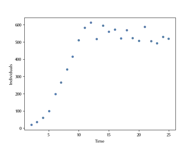
Le logistic behavior in the dataset is quite evident. It looks like the time step is always close to 1, let us see if we can approximate the integration step as constant

np.abs(df_data['Time'].diff().dropna()-1).max()

0.10359150000000028

It looks like assuming equally space data is not too bad. The integration step should be small enough to ensure that the error is not too large, we will therefore assume $h = 1/5\,.$ As we will see, this is a small enough choice, but I invite you to try with a smaller step and verify if everything is OK. We also scaled the data so that the fitted value is not too large for the numerical integration.

n_steps = 5

with pm.Model() as model:
    lam = pm.HalfNormal('lam', 2)
    kappa = pm.HalfNormal('kappa', 2)
    nu = pm.HalfNormal('nu', 0.5)
    sigma = pm.HalfNormal('sigma', 0.5)
    def f_update(n, lam, kappa, h):  # this function implements the Euler method
        return n+n*h*lam*(1-n/kappa)
    mu, update = pt.scan(fn=f_update,  # The updating function
                     outputs_info=[nu],  # The initial condition
                    non_sequences=[lam, kappa, 1/n_steps],  # The list of arguments
                    n_steps=n_steps*len(yobs))  # The number of steps
    y = pm.Normal('y', mu=mu[::n_steps], sigma=sigma, observed=yobs/100)

Since it is hard to guess a reasonable value for the parameters, it is better to take a look at the prior predictive distribution

with model:
    pr_pred = pm.sample_prior_predictive()

fig = plt.figure()
ax = fig.add_subplot(111)
for elem in az.extract(pr_pred, group='prior_predictive', var_names=['y'], num_samples=50).T:
    ax.plot(df_data['Time'], np.exp(elem.values))
ax.set_ylim([0, 200])

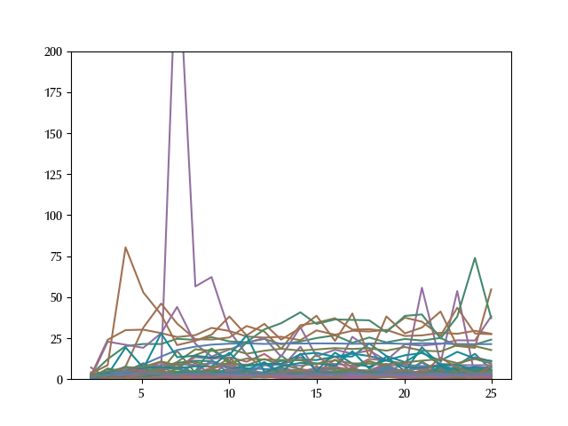
The parameters look fine, there is a fast enough growth, the limit number is large enough and the initial value covers a wide enough region. We can now fit the data.

with model:
    idata = pm.sample(nuts_sampler='numpyro', draws=2000, tune=2000, random_seed=rng)

az.plot_trace(idata)
fig = plt.gcf()
fig.tight_layout()

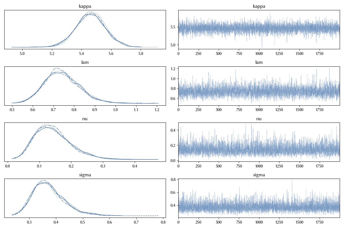
The traces look perfect, we can now inspect the posterior predictive.

with model:
    idata.extend(pm.sample_posterior_predictive(idata))
    
def fexact(x, y0, lam, k):
    y = (k*y0*np.exp(lam*x))/(k +y0*(np.exp(lam*x)-1))
    return y

dt = np.array([fexact(t, idata.posterior['nu'].values, idata.posterior['lam'].values, idata.posterior['kappa'].mean().values) 
               for t in range(len(df_data))])

ypl = dt.mean(axis=(1, 2))
fig = plt.figure()
ax = fig.add_subplot(111)
ax.fill_between(df_data['Time'], 100*idata.posterior_predictive['y'].quantile(q=0.03, dim=('draw', 'chain')),
                100*idata.posterior_predictive['y'].quantile(q=0.97, dim=('draw', 'chain')),
                alpha=0.8, color='lightgray'
               )
ax.plot(df_data['Time'], 100*idata.posterior_predictive['y'].mean(dim=('draw', 'chain')),
       color='k', ls=':')

ax.plot(df_data['Time'], ypl*100)
sns.scatterplot(df_data, x='Time', y='Individuals')

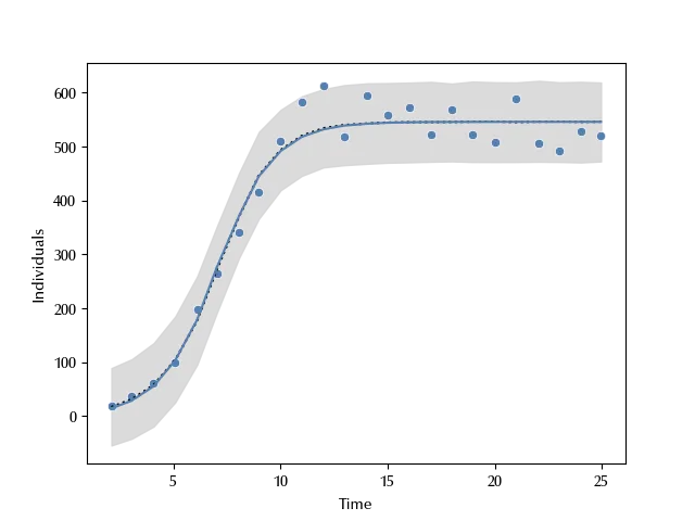
The numerical solution is identical to the analytic one, so our ODE solver does a very good job. The average looks fine, but the model provides a credible interval below 0, and this makes no sense since the number of individuals is a positive quantity. We can easily fix the above model by fitting the logarithm of the number of individuals

with pm.Model() as model_improved:
    lam = pm.HalfNormal('lam', 2)
    kappa = pm.HalfNormal('kappa', 2)
    nu = pm.HalfNormal('nu', 0.5)
    sigma = pm.HalfNormal('sigma', 0.5)
    def f_update(n, lam, kappa, h):
        return n+n*h*lam*(1-n/kappa)
    mu, update = pt.scan(fn=f_update, 
                     outputs_info=[nu],
                    non_sequences=[lam, kappa, 1/n_steps],
                    n_steps=n_steps*len(yobs))
    y = pm.Normal('y', mu=pm.math.log(mu[::n_steps]), sigma=sigma, observed=np.log(yobs/100))

with model_improved:
    idata_improved = pm.sample(nuts_sampler='numpyro',
                               draws=2000, tune=2000, random_seed=rng)

az.plot_trace(idata_improved)
fig = plt.gcf()
fig.tight_layout()

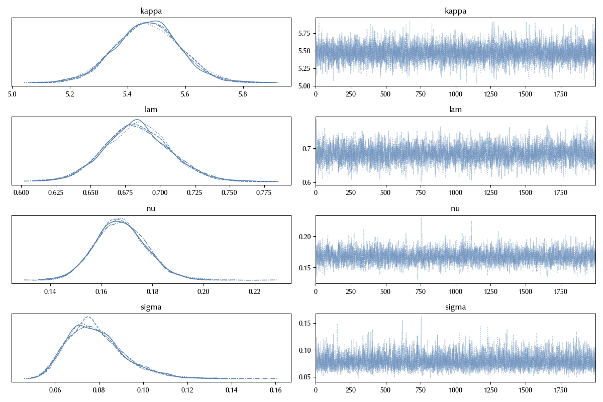
Also in this case the trace is fine. What about the posterior predictive?

with model_improved:
    idata_improved.extend(pm.sample_posterior_predictive(idata_improved))

dt_new = np.array([fexact(t, idata_improved.posterior['nu'].values, idata_improved.posterior['lam'].values, idata_improved.posterior['kappa'].mean().values) 
                   for t in range(len(df_data))])

ypl_new = dt_new.mean(axis=(1, 2))
fig = plt.figure()
ax = fig.add_subplot(111)
ax.fill_between(df_data['Time'], 100*np.exp(idata_improved.posterior_predictive['y']).quantile(q=0.03, dim=('draw', 'chain')),
                100*np.exp(idata_improved.posterior_predictive['y']).quantile(q=0.97, dim=('draw', 'chain')),
                alpha=0.8, color='lightgray'
               )
ax.plot(df_data['Time'], 100*np.exp(idata_improved.posterior_predictive['y']).mean(dim=('draw', 'chain')),
       color='k', ls=':')
ax.plot(df_data['Time'], ypl_new*100)
sns.scatterplot(df_data, x='Time', y='Individuals')

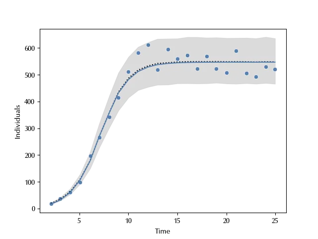
These error bars make much more sense than the previous ones, and we consider this model better than the previous one. Notice that we might decide to perform a model comparison between the two models, but I personally don’t consider this as a necessary step, since we didn’t modify the model because the fit was bad, but rather because it did not fulfill the positivity constraint.

Conclusions

With the help of pytensor’s scan function, implementing Euler algorithm has been straightforward, and the extension to any other solver is immediate. We applied this method to numerically integrate the logistic equation, and we applied it to an example from Gause’s textbook. We have also seen a little trick to impose the positivity of the solution and make the credible intervals more reasonable.

Conclusions

Suggested readings