How does MCMC works
In this post I will try and give you an idea of how does PyMC works by performing Bayesian inference from scratch. I just want to explain the underlying working principles, without entering too much into technical details, so I will try and keep things as simple as possible. This section can be safely skipped if you are not interested in understanding how MCMC works.
Sampling random numbers
The linear congruential generator
This is the simplest generator, and it allows you to generate random integers between $0$ and some large integer $c$ or, equivalently, to generate float numbers between $0$ and $1$. Given three integers $a$, $b$ and $c$, a linear congruential generator can be constructed as
import numpy as np
from matplotlib import pyplot as plt
from scipy.stats import uniform, norm, t

def rndn(x, a, b, c):
    return (a*x+b)%c
This is the default random number generator for most programming languages, and the choice of the three parameters is not unique. On the Wikipedia page you will find a large number of possible choice. A possible good one is
c = int(2**31)-1
b = int(2**29)-1
a = 17

# We initialize the sequence with a random number
seed = np.random.randint(c) % c

xtmp = [seed]
x0 = seed
for i in range(20000):
    x0 = rndn(x0, a, b, c)
    xtmp.append(x0)

fig = plt.figure(figsize=(7, 4))
ax = fig.add_subplot(111)
ax1.hist(np.array(xtmp)/c, bins=20, density=True)
fig.tight_layout()

Inverse transform sampling
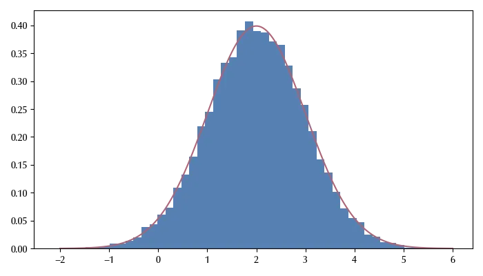
By using this generator we can sample any distribution such that the inverse of the cumulative distribution function is known. In fact, if $X$ is distributed according to the uniform distribution over \([0, 1]\) and $F(x)$ is the cumulative distribution function of a distribution with probability density $p(x)\,,$ then $F^{-1}(X)$ is distributed according to \(p(x)\,.\)
Let us take as an example the normal distribution function with mean $2$
xpl = np.linspace(-2, 6, 200)
fig = plt.figure(figsize=(7, 4))
ax = fig.add_subplot(111)
ax.hist(norm(loc=2).ppf(np.array(xtmp)/c), bins=50, density=True)
ax.plot(xpl, norm(loc=2).pdf(xpl))
fig.tight_layout()

As you can see, the theoretical distribution matches the sampled one with quite a high accuracy. There is, of course, the issue that we are sampling correlated numbers, while we would like to have independent random numbers. This is one of the central problems of any random number generator, and the easiest way to deal with is to take a slice of the sampled array, since the correlation between distant elements is smaller than the one between nearby elements.
Markov Chain Monte Carlo
The inverse transform sampling only works with distributions with known cumulative distribution function. When we perform Bayesian statistics, however, we don’t know how to compute it, so other methods are needed. Here we will introduce the Markov Chain Monte Carlo (MCMC) techniques. These methods rely on properties of Markov processes, and a discussion on this topic is far away from the subject of this blog, so we will limit ourselves to the illustration of the methods.
The Metropolis algorithm
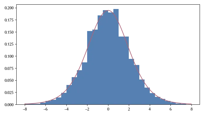
The Metropolis algorithm allows you to sample any distribution with known density/mass function, you only need a proposal distribution. The algorithm can be implemented as follows:
def prop(xold: float, scale: float, logpdf):
    # The proposal distribution
    xtemp = np.random.normal(loc=0, scale=scale)
    log_w = logpdf(xtemp) - logpdf(xold)
    if log_w > 0:
        return xtemp
    else:
        w = np.exp(log_w)
        z = np.random.uniform(low=0, high=1)
        if z < w:
            return xtemp
        else:
            return xold
Let us now see how to use it
# Our initial point
x0 = np.random.normal(loc=0, scale=2)

# Our target distribution
target = t(df=10, loc=0, scale=2).logpdf


res = []
for n in range(50000):
    x0 = prop(x0, 12, target)
    res.append(x0)

# We discard the first half of the sample, since
# the initial points may be far away from the target distribution
sz = int(len(res)//2)

# We only take a subsample to reduce the correlation
res = res[sz::3]

fig = plt.figure()
ax = fig.add_subplot(111)
xpl = np.arange(-8, 8, 3e-2)
ax.hist(res, bins=np.arange(-8, 8, 0.5), density=True)
ax.plot(xpl, np.exp(target(xpl)))
fig.tight_layout()

The Hamiltonian Monte Carlo algorithm
For the Metropolis algorithm, the success of the sampling crucially depends on the proposal distribution, and this might cause problems for strongly correlated high dimensional distributions. For this reason, the best algorithm for high dimensional distributions is the Hamiltonian Monte Carlo (HMC). The underlying idea behind the HMC is that, if $x$ is distributed according to \(f(x)\) then
\[g(p, x) = \frac{1}{\sqrt{2 \pi}} e^{-p^2/2} p(x)\]has \(p(x)\) as marginal distribution. If we then observe that
\[-\log(g(p, x)) = \frac{p^2}{2} - \log(p(x)) + \log{\sqrt{2\pi}}= H(p, x)\]describes the hamiltonian of a particle with potential \(-\log(p(x))\,.\) Thanks to this, it is possible to prove that the following algorithm produces a sample distributed according to \(p(x):\)
def leapfrog(xold, p, dt, potential, eps):
    p1 = p - dt/2*(potential(xold+eps)-potential(xold))/eps
    xn = xold + dt*p1
    p2 = p1 - dt/2*(potential(xn+eps)-potential(xn))/eps
    return p2, xn

def hamiltonian(x, p, potential):
    return p**2/2 + potential(x)

p0 = np.random.normal(10)
x0 = np.random.normal(10)

L = 1
dt = 0.5
eps = 1e-4

def pot(x):
    return -target(x)

xn = x0
rs = []
for k in range(50000):
    pn = np.random.normal(loc=0, scale=1)
    for s in range(L):
        ptmp, xtmp = leapfrog(xn, pn, dt, pot, eps)
        w = np.random.uniform(low=0, high=1)
        alpha = np.min([1, np.exp(-hamiltonian(xtmp, ptmp, pot)+hamiltonian(xn, pn, pot))])
        if w < alpha:
            xn = xtmp
        rs.append(xn)

fig = plt.figure(figsize=(7, 4))
ax = fig.add_subplot(111)
xpl = np.arange(-8, 8, 3e-2)
ax.hist(rs[20000::5], bins=np.arange(-8, 8, 0.5), density=True)
ax.plot(xpl, np.exp(target(xpl)))

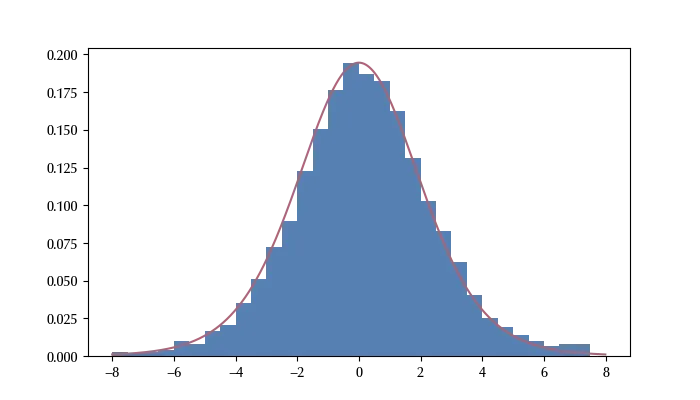
This method works much better than the Metropolis algorithm, especially for highly correlated variables. Up to few years ago, this method was not very popular because implementing it requires the computation of the Jacobian matrix (the derivative of the log pdf). In the 2010s, however, automatic differentiation became available, and it became possible to implement this algorithm within STAN and many other frameworks to perform Bayesian statistics. These frameworks allow the user to sample the posterior by simply specifying the mathematical model in a natural way.
Bayesian inference with HMC
We can now leverage what we implemented above to compute the posterior distribution of a one dimensional system. Let us assume that we have some data, and we know that it is distributed according to a Student-t distribution with 5 dof and parameter $\sigma=1\,,$ but we don’t know its mean. What we know is that the mean’s order of magnitude is roughly 1.
# Sample the fake data
data = 0.8 + np.random.standard_t(df=5, size=500)

# We now implement Bayes theorem.
# We take as prior for our parameter a normal distribution with sigma=20

def post(x):
    likelihood = t(df=5, loc=x, scale=1).logpdf(data)
    prior = norm(loc=0, scale=20).logpdf(x)
    return -np.sum(likelihood) - prior

xn = np.random.normal(loc=0, scale=2)
rs = []
dtn = 1e-2
for k in range(20000):
    pn = np.random.normal(loc=0, scale=1)
    for s in range(L):
        ptmp, xtmp = leapfrog(xn, pn, dtn, post, eps)
        w = np.random.uniform(low=0, high=1)
        alpha = np.min([1, np.exp(-hamiltonian(xtmp, ptmp, post)+hamiltonian(xn, pn, post))])
        if w < alpha:
            xn = xtmp
        rs.append(xn)

trace = rs[2000::5]
fig = plt.figure()
ax = fig.add_subplot(111)
ax.hist(trace, density=True, bins=30)

We can now easily compute any estimate for the parameter.
np.mean(trace)
np.quantile(trace, 0.03)
np.quantile(trace, 0.96)
We can therefore conclude that our parameter has mean 0.88 and 94% credible interval \([0.78, 0.97]\,.\)
Conclusion
I hope I managed to give you an idea of how does a probabilistic programming language works. In the next posts we will see how to use PyMC to write down statistical models and criticize them.
