
Nested factor
A situation when mixed models can make the difference is when you are dealing with nested factors. Think about an experiment where the standard teaching method is applied to classes A to D of school 1 and 2 while an innovative teaching method is applied to classes A to D of school 3 and 4.
When we assess the effectiveness of the method, we must both take into account the school effect and the class effect. In doing so, however, we must include the fact that class A from school 1 is different from class A from school 2, 3 and 4. In other words, classval is nested within school.
This is straightforward to do in Bambi, and we are going to show how to do so.
The pastes dataset
Here we will use the pastes dataset from the lme4 R repo. As explained in the documentation
The data are described in Davies and Goldsmith (1972) as coming from “ deliveries of a chemical paste product contained in casks where, in addition to sampling and testing errors, there are variations in quality between deliveries … As a routine, three casks selected at random from each delivery were sampled and the samples were kept for reference. … Ten of the delivery batches were sampled at random and two analytical tests carried out on each of the 30 samples”.
The dataset can be downloaded from this link.
import pandas as pd
import seaborn as sns
import numpy as np
import pymc as pm
import arviz as az
import bambi as bmb
from matplotlib import pyplot as plt

rng = np.random.default_rng(42)

kwargs = {'nuts_sampler': 'numpyro', 'random_seed': rng,
          'draws': 2000, 'tune': 2000, 'chains': 4, 'target_accept': 0.95}

df = pd.read_csv('pastes.csv')

df.head()
| Unnamed: 0 | strength | batch | cask | sample | |
|---|---|---|---|---|---|
| 0 | 1 | 62.8 | A | a | A:a |
| 1 | 2 | 62.6 | A | a | A:a |
| 2 | 3 | 60.1 | A | b | A:b |
| 3 | 4 | 62.3 | A | b | A:b |
| 4 | 5 | 62.7 | A | c | A:c |
fig, ax = plt.subplots()
sns.scatterplot(df, hue='cask', x='batch', y='strength', ax=ax)
fig.tight_layout()
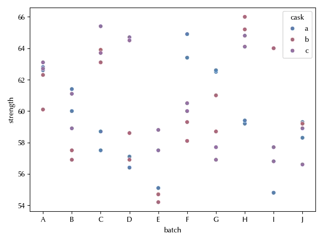
Here we want to quantify the average strength as well as the variability, and we have two sources ov variability, the batch and the cask. The cask is however nested within the batch, since cask a from batch A is not the same as cask a from batch B.
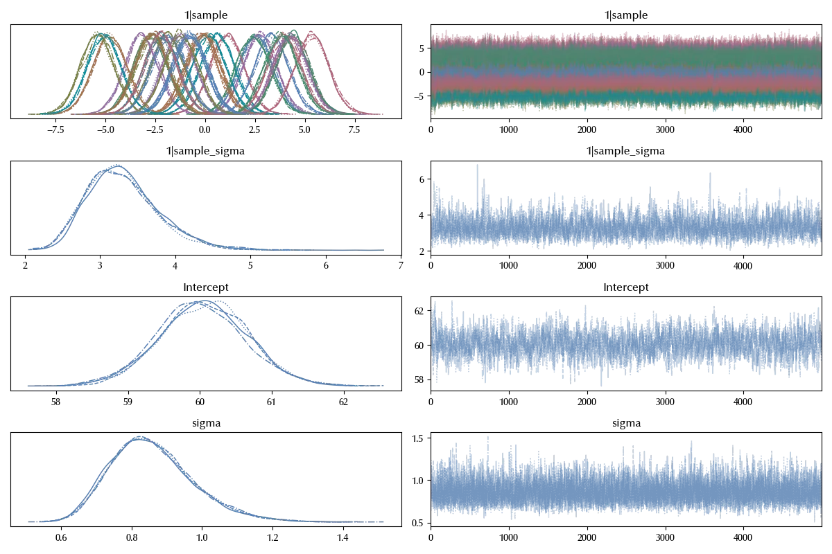
The first way to account for this is to use the sample column:
model_easy = bmb.Model('strength ~ 1 + (1|sample)', data=df)

idata_easy = model_easy.fit(**kwargs)

az.plot_trace(idata_easy)
fig = plt.gcf()
fig.tight_layout()
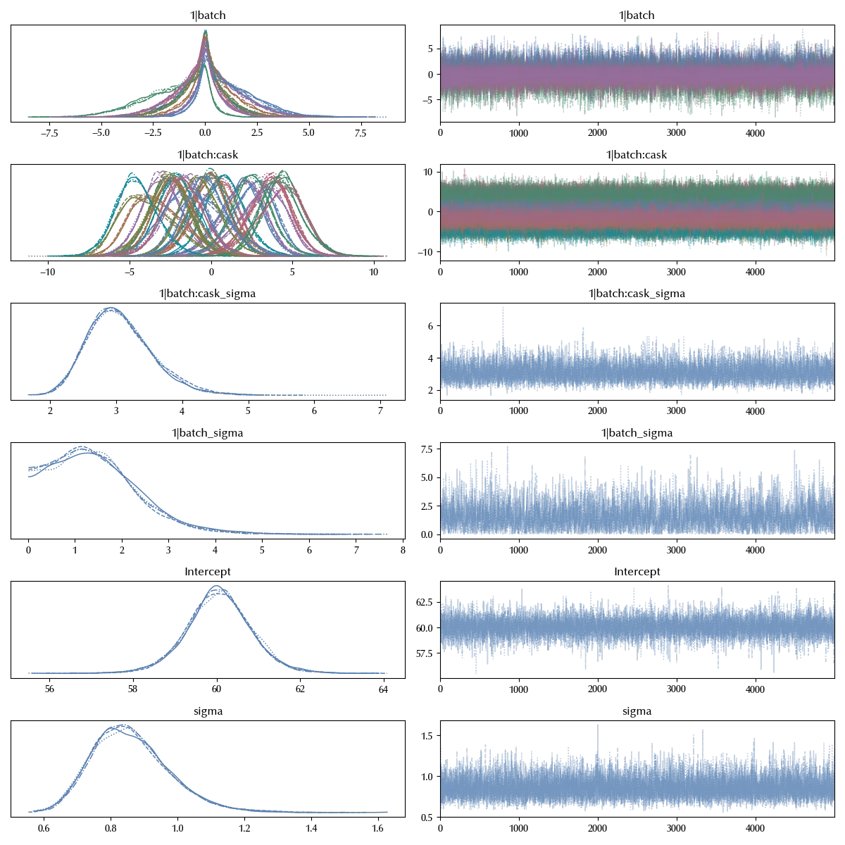
The second way is to use the \ operator in Bambi. While in this case the two approaches are equivalent, as soon as the number of columns grows and the model complexity increases, creating additional columns becomes cumbersome and an appropriate syntax becomes very helpful.
model = bmb.Model('strength ~ (1 | batch/cask )', data=df)

idata = model.fit(**kwargs)

az.plot_trace(idata)
fig = plt.gcf()
fig.tight_layout()
In order to convince you that the two models are equivalent, let us inspect the summary of the models
az.summary(idata_easy, var_names=['Intercept', 'sigma'])
| mean | sd | hdi_3% | hdi_97% | mcse_mean | mcse_sd | ess_bulk | ess_tail | r_hat | |
|---|---|---|---|---|---|---|---|---|---|
| Intercept | 60.049 | 0.618 | 58.899 | 61.233 | 0.017 | 0.012 | 1306 | 2558 | 1 |
| sigma | 0.86 | 0.118 | 0.655 | 1.087 | 0.001 | 0.001 | 6801 | 9953 | 1 |
az.summary(idata, var_names=['Intercept', 'sigma'])
| mean | sd | hdi_3% | hdi_97% | mcse_mean | mcse_sd | ess_bulk | ess_tail | r_hat | |
|---|---|---|---|---|---|---|---|---|---|
| Intercept | 60.052 | 0.793 | 58.539 | 61.522 | 0.008 | 0.006 | 10081 | 11314 | 1 |
| sigma | 0.86 | 0.116 | 0.652 | 1.073 | 0.001 | 0.001 | 7556 | 11062 | 1 |
As we anticipated, the parameters of the two models give identical estimates for these parameters within the MC error.
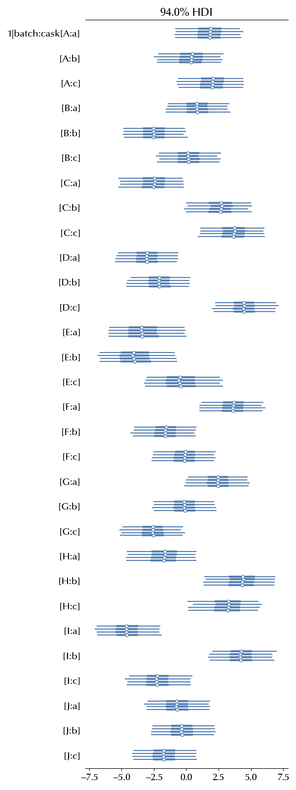
Let us now inspect the cask effect
az.plot_forest(idata, var_names=['1|batch:cask'])
fig = plt.gcf()
fig.tight_layout()
Conclusions
Nested factors are a common source of mistakes, and you should always keep in mind that having the same name does not imply being the same thing.
Once you correctly identify them, implementing them in Bambi is straightforward.
%load_ext watermark
%watermark -n -u -v -iv -w -p xarray,pytensor,numpyro
Python implementation: CPython
Python version : 3.12.8
IPython version : 8.31.0
xarray : 2024.11.0
pytensor: 2.26.4
numpyro : 0.16.1
seaborn : 0.13.2
matplotlib: 3.10.0
arviz : 0.20.0
bambi : 0.15.0
pymc : 5.19.1
numpy : 1.26.4
pandas : 2.2.3
Watermark: 2.5.0