
Repeated measures
The split-plot design is helpful when we want to determine the effect of one (or more than one) treatment over time and the same measure is repeated on a unit at different times, as we will show here.
We can consider the unit as the whole plot, while the measurements taken at different times as the sub-plots.
Here we will show how to perform this kind of analysis with a dataset coming from the (already cited) Design and Analysis of Experiments with R textbook by John Lawson. The dataset can be found at this link.
import pandas as pd
import seaborn as sns
import numpy as np
import pymc as pm
import arviz as az
import bambi as bmb
from matplotlib import pyplot as plt

rng = np.random.default_rng(42)

kwargs = {'nuts_sampler': 'numpyro', 'random_seed': rng, 'draws': 2000, 'tune': 2000, 'chains': 4, 'target_accept': 0.95,
         'idata_kwargs': dict(log_likelihood = True)}

df = pd.read_csv('/home/stippe/Downloads/dairy.csv')

df.rename(columns={'Unnamed: 0': 'cow'}, inplace=True)

df.head()
| cow | Diet | pr1 | pr2 | pr3 | pr4 | |
|---|---|---|---|---|---|---|
| 0 | 1 | Barley | 3.63 | 3.57 | 3.47 | 3.65 |
| 1 | 2 | Barley | 3.24 | 3.25 | 3.29 | 3.09 |
| 2 | 3 | Barley | 3.98 | 3.6 | 3.43 | 3.3 |
| 3 | 4 | Barley | 3.66 | 3.5 | 3.05 | 2.9 |
| 4 | 5 | Barley | 4.34 | 3.76 | 3.68 | 3.51 |
Here the first column represents the cow, the second column the diet, while the remaining four columns represent the protein percentage of the milk measured at four different weeks.
This format is not useful, so it’s better to melt the above dataset
df_melt = df.melt(value_vars=['pr1', 'pr1', 'pr3', 'pr4'],
                  var_name='week', value_name='protein', id_vars=['cow', 'Diet'])

df_melt['x'] = df_melt['week'].str[2].astype(int)

df_melt.head()
| cow | Diet | week | protein | x | |
|---|---|---|---|---|---|
| 0 | 1 | Barley | pr1 | 3.63 | 1 |
| 1 | 2 | Barley | pr1 | 3.24 | 1 |
| 2 | 3 | Barley | pr1 | 3.98 | 1 |
| 3 | 4 | Barley | pr1 | 3.66 | 1 |
| 4 | 5 | Barley | pr1 | 4.34 | 1 |
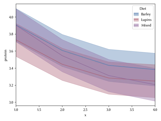
fig, ax = plt.subplots()
sns.lineplot(df_melt, y='protein', x='x', hue='Diet', ax=ax)
ax.set_xlim([1, 4])
fig.tight_layout()
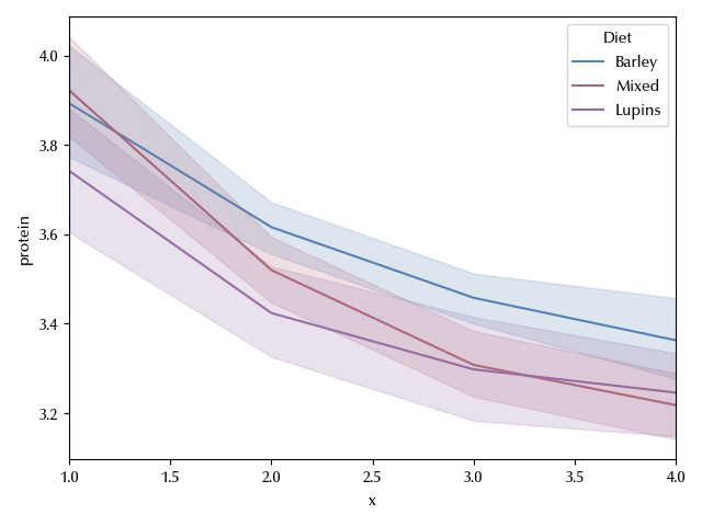
There is a clear time dependence, and it also looks like it’s possibly non-linear. From what we said before, it’s straightforward to implement the split-plot design to this dataset.
categorical = ['cow','Diet','week']

model = bmb.Model('protein ~ Diet*week + (1 | cow:Diet)',
                  data=df_melt, categorical=categorical)

idata = model.fit(**kwargs)
fig, ax = plt.subplots()
az.plot_forest(idata, var_names=['1|cow:Diet_sigma', 'Diet'], ax=ax)
fig.tight_layout()
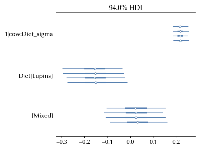
From the above figure we see that the diet effect is less than the cow variability, so changing the diet would have an impact which has a negligible practical impact.
We may also ask what’s the impact of discretizing a continuous variables as the time, and this is generally considered suboptimal. We can however easily implement the continuous-time version of the above model. We will use a diet level slope, and an overall quadratic effect to account for possible non-linearity.
model_cont = bmb.Model('protein ~1 + Diet*x + I(x**2) + (1 | cow:Diet)',
data=df_melt, categorical=categorical)
idata_cont = model_cont.fit(**kwargs)
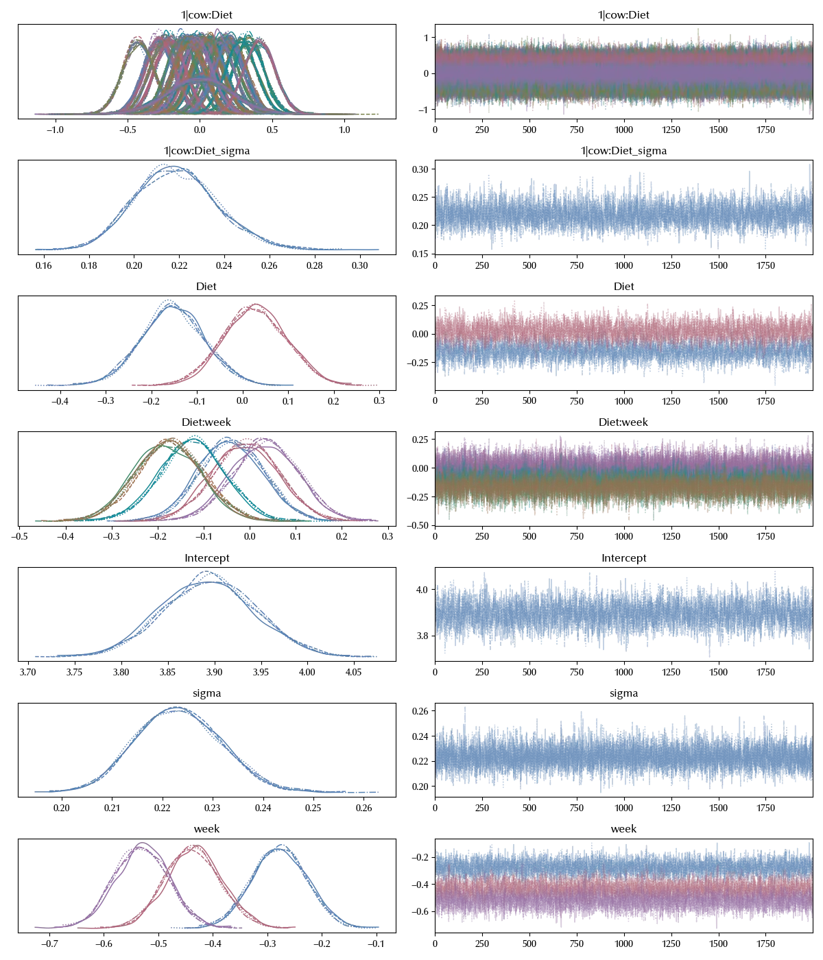
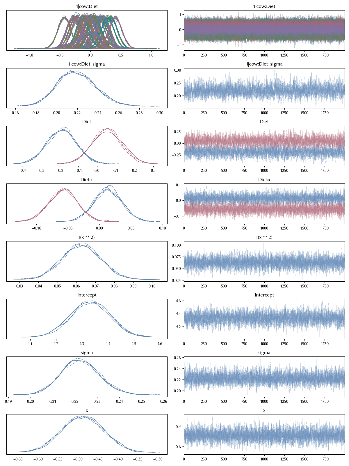
az.plot_trace(idata_cont)
fig = plt.gcf()
fig.tight_layout()
Let us now compare the two models
df_comp = az.compare({'discrete': idata, 'continuous': idata_cont})

df_comp
| rank | elpd_loo | p_loo | elpd_diff | weight | se | dse | warning | scale | |
|---|---|---|---|---|---|---|---|---|---|
| continuous | 0 | -16.2897 | 94.8413 | 0 | 1 | 13.8243 | 0 | False | log |
| discrete | 1 | -20.4463 | 98.4776 | 4.15654 | 1.73195e-14 | 14.0241 | 1.77448 | True | log |
fig, ax = plt.subplots()
az.plot_compare(df_comp, ax=ax)
fig.tight_layout()
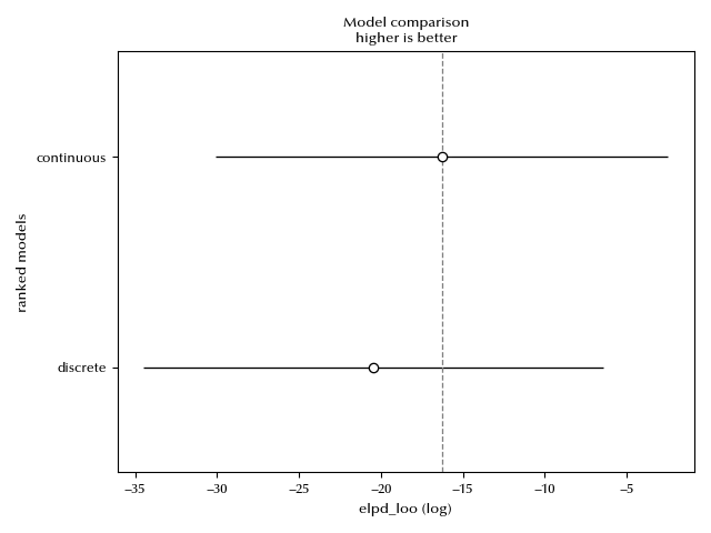
The continuous model is slightly better than the discrete one.
With Bambi we can easily plot the posterior predictive distribution
fig, ax = plt.subplots()
bmb.interpret.plot_predictions(model=model_cont, idata=idata_cont, average_by=['x','Diet'], ax=ax)
ax.set_xlim([1, 4])
fig.tight_layout()
Conclusions
We have seen how we can use mixed effect models to model repeated measurements in a completely randomized design. We have also seen how to implement models with continuous variables by using Bambi.
%load_ext watermark
%watermark -n -u -v -iv -w -p xarray,numpyro,jax,jaxlib
Python implementation: CPython
Python version : 3.12.8
IPython version : 8.31.0
xarray : 2024.11.0
numpyro: 0.16.1
jax : 0.4.38
jaxlib : 0.4.38
bambi : 0.15.0
pandas : 2.2.3
arviz : 0.20.0
seaborn : 0.13.2
matplotlib: 3.10.0
numpy : 1.26.4
pymc : 5.19.1
Watermark: 2.5.0