Split plot design

There are contexts where a complete randomization of the treatment assignment is not convenient enough to justify a full factorial experiment, and a split-plot design is often a good alternative.

Split plot designs have been invented in agriculture, where a field (the “full plot”) is divided into split-plots. Assume that you have two factors of interest, the irrigation method and the fertilizer. While the fertilizer can be easily changed across sub-plots, it’s hard to do the same for the irrigation method by ensuring that the treatment is uniform across the entire field. This is a classical example of split-plot design, where you have a hard-to-change factor (the irrigation method) and an easy-to-change factor (the fertilizer).

Other situations where you should consider the split-plot design is when changing one of the factors requires a lot of time or effort, and in this case the factor might be treatment as a plot factor. A typical example is the temperature: you should cool down and re-heat the environment to the randomly assigned temperature in order to properly treat it as randomized, and this is often not practically feasible due to time constraints.

If we treat this experiment as a full factorial example, we would underestimate the uncertainty of our treatment effects, since we are not randomly assigning the irrigation to the different subplots.

Since the irrigation is randomly assigned to the different plot, we can model the plot level treatment effect as follows:

\[\begin{align} y_{iu} \sim & \alpha_i + \eta_{iu} \\ \eta_{iu} \sim & \mathcal{N}(0, \sigma_P) \end{align}\]

where $\alpha_i$ is the irrigation effect and $\eta_iu$ is the noise term and $y_{iu}$ the average outcome at the plot level. We can then include the fertilizer effect

\[\begin{align} y_{iujt} \sim & \alpha_i + \eta_{iu} + \beta_j + (\alpha \beta)_{ij} + \varepsilon_{iujt} \\ \eta_{iu} \sim & \mathcal{N}(0, \sigma_P) \\ \eta_{iujt} \sim & \mathcal{N}(0, \sigma_S) \end{align}\]

We can easily implement the above model by using a hierarchical model, where we add a random intercept grouping at the plot level. Above we assumed a full interaction model between the fertilizer and the irrigation method. Let us take a look at the fertilizer dataset by Julian Faraway. The dataset has unknown source and has been found by Faraway online.

An application

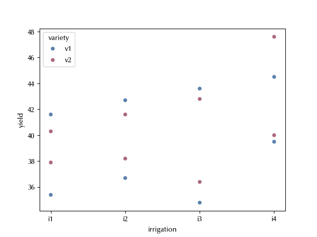
The experiment is almost identical to the one described above, except that the split-plot factor is not the fertilizer but the crop variety. This dataset has been analyzed in R in this website, here we will only bring it to python with minor modifications.

import pandas as pd
import seaborn as sns
import numpy as np
import pymc as pm
import arviz as az
import bambi as bmb
from matplotlib import pyplot as plt

rng = np.random.default_rng(42)

kwargs = {'nuts_sampler': 'numpyro', 'random_seed': rng,
          'draws': 2000, 'tune': 2000, 'chains': 4,
          'target_accept': 0.95}

df = pd.read_csv('data/irrigation.csv')

df

	field	irrigation	variety	yield
1	f1	i1	v1	35.4
2	f1	i1	v2	37.9
3	f2	i2	v1	36.7
4	f2	i2	v2	38.2
5	f3	i3	v1	34.8
6	f3	i3	v2	36.4
7	f4	i4	v1	39.5
8	f4	i4	v2	40
9	f5	i1	v1	41.6
10	f5	i1	v2	40.3
11	f6	i2	v1	42.7
12	f6	i2	v2	41.6
13	f7	i3	v1	43.6
14	f7	i3	v2	42.8
15	f8	i4	v1	44.5
16	f8	i4	v2	47.6

The scatterplot of the irrigation dataset

model = bmb.Model('yield ~ irrigation*variety + (1|field)',
                  data=df, categorical=['field', 'irrigation', 'variety'])

idata = model.fit(**kwargs, idata_kwargs=dict(log_likelihood = True))

az.plot_trace(idata)
fig = plt.gcf()
fig.tight_layout()

The trace of the above model

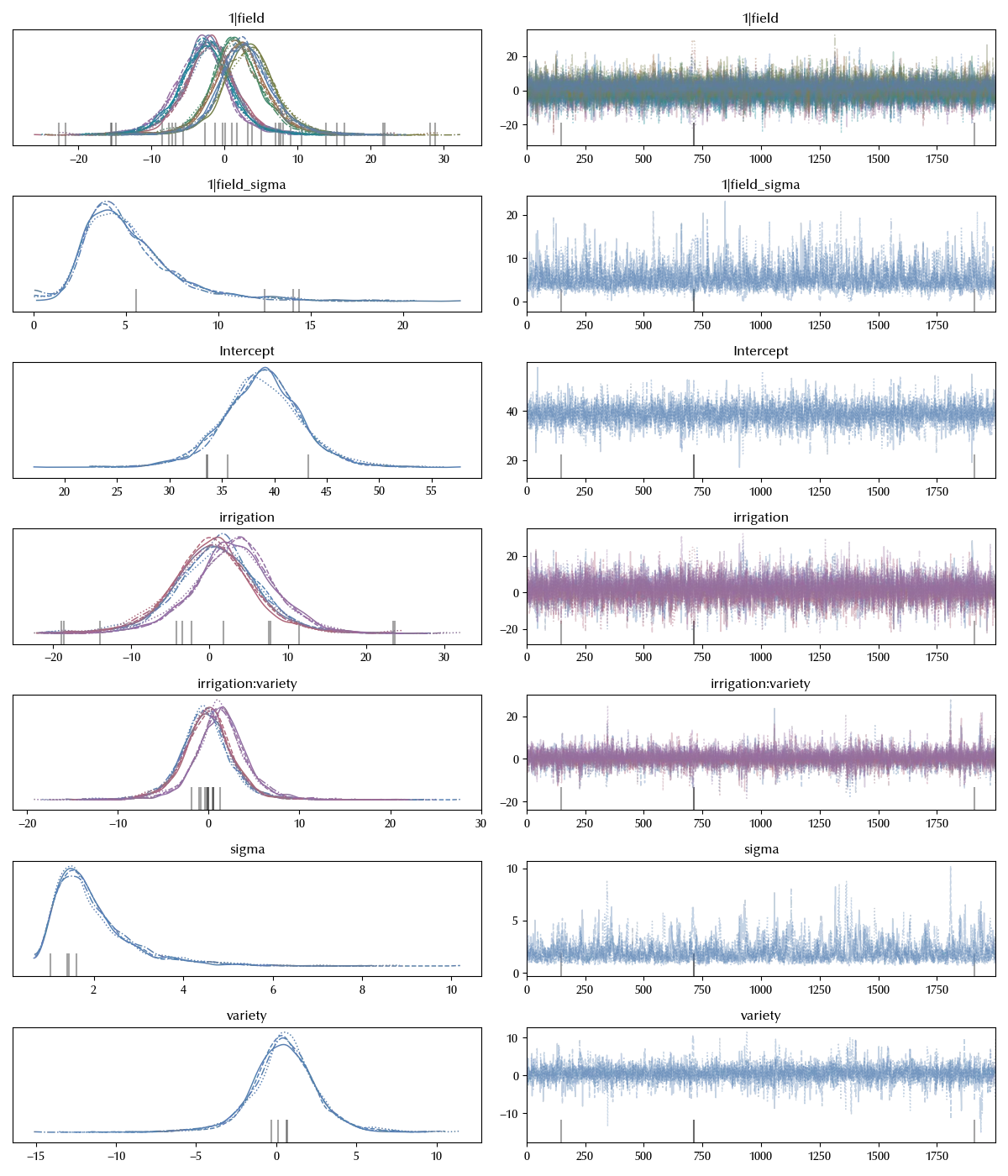
The trace doesn’t show any big issue. Let us take a look at the effects.

fig, ax = plt.subplots()
az.plot_forest(idata, var_names=['irrigation','irrigation:variety', 'variety'], ax=ax)
fig.tight_layout()

The main effects of the above model

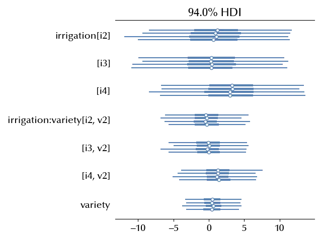
The presence of an effect is not clear, and since the interaction term is compatible with zero, we can see what a non-interacting model tells us.

model_red = bmb.Model('yield ~ irrigation + variety + (1|field)',
                      data=df, categorical=['field', 'irrigation', 'variety'])

idata_red = model_red.fit(**kwargs, idata_kwargs=dict(log_likelihood = True))

az.plot_trace(idata_red)
fig = plt.gcf()
fig.tight_layout()

The trace of the reduced model

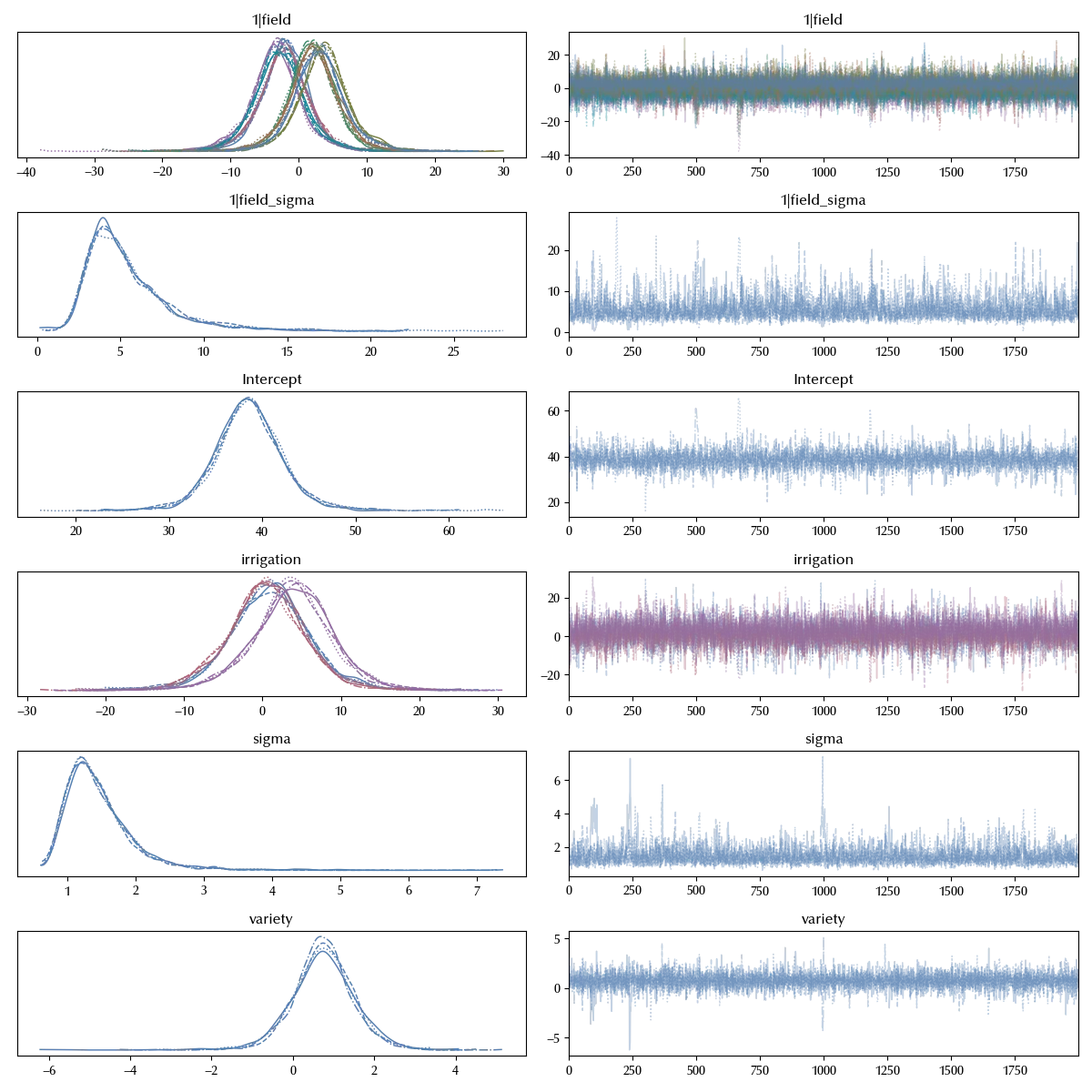
Also in this case the traces are fine.

Let us first of all verify if the non-interacting model is appropriate

df_comp = az.compare({'full': idata, 'interaction-free': idata_red})
df_comp

	rank	elpd_loo	p_loo	elpd_diff	weight	se	dse	warning	scale
interaction-free	0	-33.4474	8.38432	0	1	1.21474	0	True	log
full	1	-40.5167	11.725	7.06935	5.24025e-14	0.736522	1.11308	True	log

az.plot_compare(df_comp)

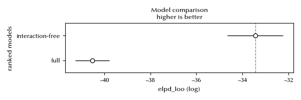
There are no doubts that the non-interacting model is appropriate. Let us take a closer look at the variety effect.

az.plot_posterior(idata_red, var_names=['variety'])
fig = plt.gcf()
fig.tight_layout()

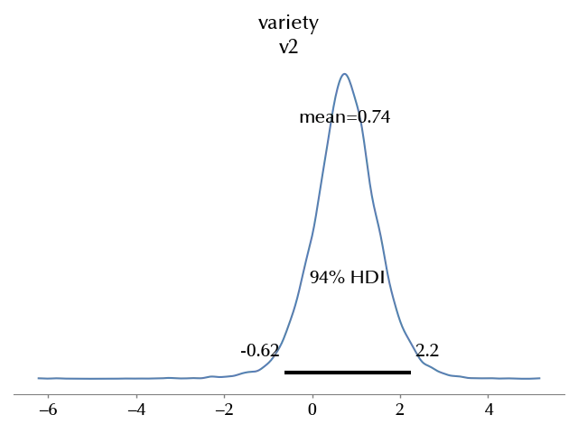
Apparently there might be an effect, but our uncertainties are too large for a clear conclusion.

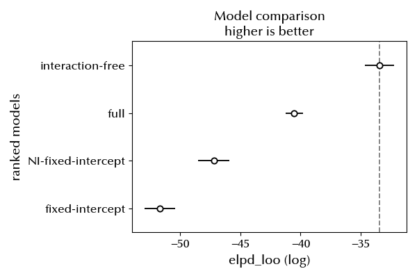
Notice that $\sigma_{1|field}$ is much larger than $\sigma$, so it would be a mistake to neglect the random intercept part.

model_nr = bmb.Model('yield ~ irrigation + variety', data=df, categorical=['field', 'irrigation', 'variety'])
idata_nr = model_nr.fit(**kwargs, idata_kwargs=dict(log_likelihood = True))
model_nr_int = bmb.Model('yield ~ irrigation * variety', data=df, categorical=['field', 'irrigation', 'variety'])
idata_nr_int = model_nr_int.fit(**kwargs, idata_kwargs=dict(log_likelihood = True))

df_comp_new = az.compare({'full': idata,
                          'interaction-free': idata_red,
                          'NI-fixed-intercept': idata_nr,
                          'fixed-intercept': idata_nr_int})

az.plot_compare(df_comp_new)
fig = plt.gcf()
fig.tight_layout()

%load_ext watermark
%watermark -n -u -v -iv -w -p xarray,pytensor,numpyro

Conclusions

We discussed how to recognize and analyze a split-plot experiment by using mixed effect models with PyMC, Arviz and Bambi. We discussed the pros and cons of this design with a practical example.

An application

Conclusions

Suggested readings