Crossover design

A common application of the latin square design is the crossover design. In this design we apply the same set of treatments by changing the order to different groups. In the simplest case, when only two treatments A and B are studied, we have that group 1 first get treatment A and then treatment B, while group 2 has first treatment B then A. The outcome is measured after each treatment, and between the treatment we wait a time named the washout time.

The underlying model is assumed as follows:

\[y_{ijk} \sim \mathcal{N}( \alpha_i + \beta_j + \tau_k, \sigma)\]

where $\alpha_i$ represents the effect of treatment $i$, $\beta_j$ represents the effect of period $j$ and $\tau_k$ is the individual effect (which is our blocking factor).

We will take the individual effect as a hierarchical effect. If we rename $\mu = \alpha_1 + \beta_1$ we can redefine $\delta$ as the difference between the two treatment effects, while the difference between the two period effects as $\gamma$.

We can easily implement the above model, as shown below. We will use a dataset taken from this tutorial where the crossover design is explained in great detail.

import pandas as pd
import seaborn as sns
import numpy as np
import pymc as pm
import arviz as az
import bambi as bmb
from matplotlib import pyplot as plt

rng = np.random.default_rng(42)

kwargs = {'nuts_sampler': 'numpyro', 'random_seed': rng,
          'draws': 2000, 'tune': 2000, 'chains': 4}

df = pd.read_csv('data/chowliu73_crossover.csv')

df.head()

	p1	p2
0	74.675	73.675
1	96.4	93.25
2	101.95	102.125
3	79.05	69.45
4	79.05	69.025

First of all, we will bring the data in a more convenient format.

df['ind'] = df.index

df_melt = df.melt(value_vars=['p1', 'p2'], var_name='period', id_vars=['ind', 'seq'])

df_melt['trt']=(df_melt['period'].str[1].astype(int)-1)*(1-df_melt['seq']) 
+ (1-(df_melt['period'].str[1].astype(int)-1))*(df_melt['seq'])

df_melt['trt']=((df_melt['period'].str[1].astype(int)-1)*(1-df_melt['seq']) 
                + (1-(df_melt['period'].str[1].astype(int)-1))*(df_melt['seq']))

df_melt[['seq', 'period', 'trt']].drop_duplicates().pivot(index='period', columns='seq', values='trt')

period	seq=0	seq=1
p1	0	1
p2	1	0

In the above table we show the treatment received during a period from the group seq. We can now immediately implement the latin square model, where we will consider the individual effect as a random effect.

model_bmb = bmb.Model('value ~ 1 + trt + (1|ind) + period', data=df_melt, categorical=['ind', 'trt', 'period'])

idata_bmb = model_bmb.fit(**kwargs)

az.plot_trace(idata_bmb)
fig = plt.gcf()
fig.tight_layout()

The trace of the above model

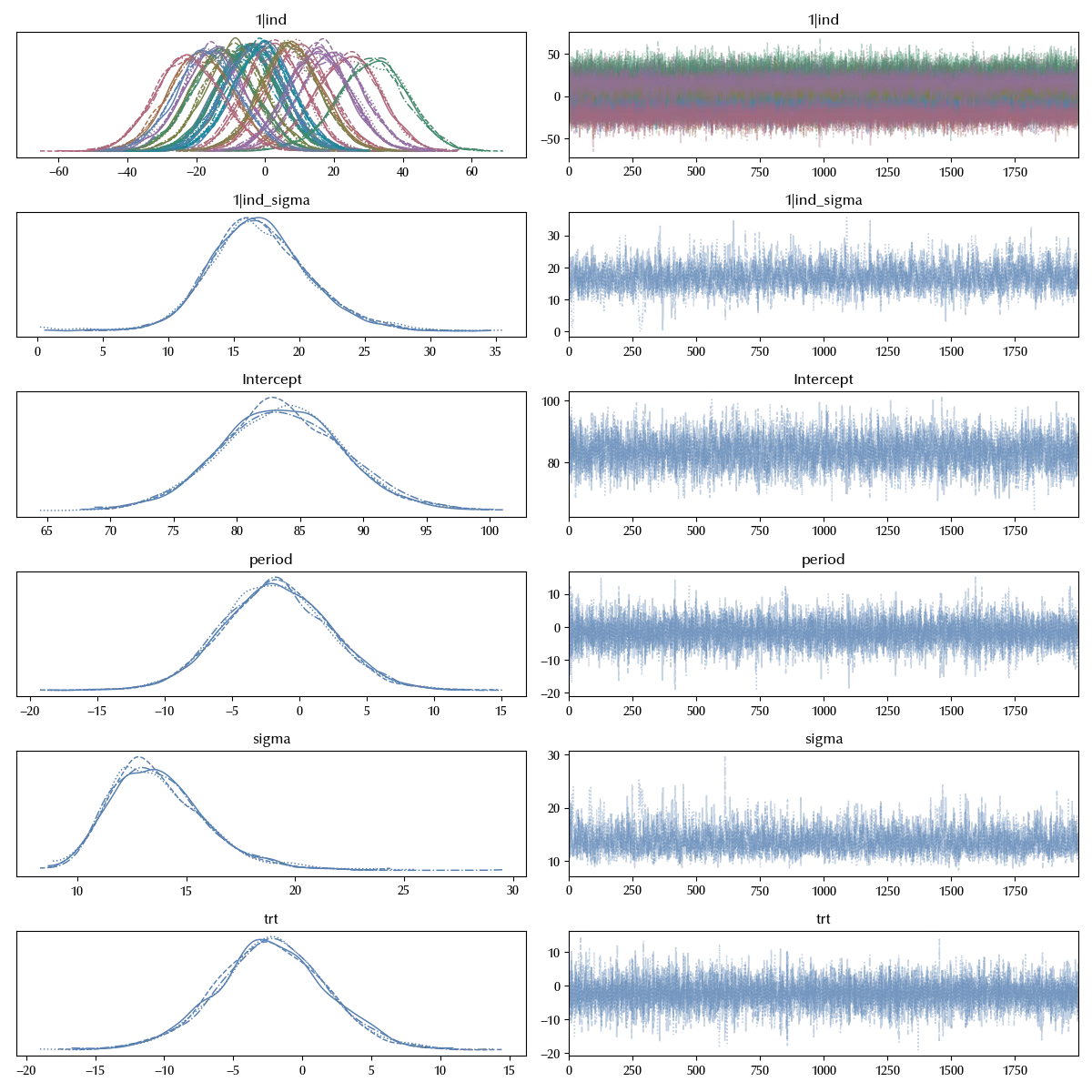
az.summary(idata_bmb, var_names=['delta', 'gamma'])

	mean	sd	hdi_3%	hdi_97%	mcse_mean	mcse_sd	ess_bulk	ess_tail	r_hat
trt[1]	-2.261	4.028	-9.508	5.807	0.037	0.043	12080	5873	1
period[p2]	-1.719	3.994	-9.403	5.512	0.038	0.047	11223	5599	1

As we can see, nor the treatment neither the period show a relevant impact on the outcome.

Suggested readings