Latin square design

The randomized block design can be easily generalized to two or more blocking factors. However, if the experimental runs are slow, it might not be convenient to run all possible combinations for all the blocks, since we are not interested in finding the dependence of the outcome variable on the blocking factors. If the number of treatment levels is equal to the number of levels of both blocking factors, a popular design with two blocking factors is the latin square design. In this design, each treatment level is tested against each level of each blocking factor once.

The latin square design

An $n\times n$ latin square is an $n \times n$ matrix where to each matrix element is assigned a letter (or a number, or any unique symbol) $a_1,…a_n$ and each letter only appears once for each row and each column. As ane example, a $3 \times 3$ latin square could be

\[\begin{pmatrix} A & B & C \\ C & A & B \\ B & C & A \\ \end{pmatrix}\]

The randomization can be achieved by first applying a random permutation to the rows and then applying a random permutation to the columns. The entire construction can be performed as follows:

import numpy as np

def latin_square(n):
    r = list(range(n))
    out = []
    for j in range(n):
        row = r[j:]+r[:j]
        out += [row]
    mat = np.array(out)
    p1 = np.random.permutation(n)
    p2 = np.random.permutation(n)
    m1 = mat[p1]
    m2 = (m1.T)[p2].T
    return m2

If we only perform one repetition for each setting, we have 9 runs, and this is enough to fit a linear non-interacting model. The interaction terms, however, cannot be estimated by using this model. Of course, allowing for multiple repetitions would not change the above situation, and it only allows us to have a more precise estimate of our parameters. The model for the latin square can be written as

\[y_{ijk} \sim \mathcal{N}(\mu_{ijk}, \sigma)\]

where

\[\mu_{ijk} = \alpha_i + \beta_j + \delta_k\]

and $i,j,k\in \left\{1,2,3\right\}$ correspond to the row effect, the column effect and the treatment effect respectively.

Our experiment

In the following experiment we will use a latin square experiment to compare the training time of three algorithms by blocking on the train-test seed and on the training order.

import random
import time
import pandas as pd
import numpy as np
from ucimlrepo import fetch_ucirepo
from sklearn.linear_model import RidgeClassifier
from sklearn.model_selection import train_test_split
from sklearn.ensemble import RandomForestClassifier
from sklearn.linear_model import LogisticRegression
from sklearn.svm import LinearSVC
from sklearn.linear_model import RidgeClassifier
from sklearn.naive_bayes import BernoulliNB, GaussianNB
from sklearn.neighbors import NearestCentroid

dataset = fetch_ucirepo(id=942)

Xs = dataset.data.features
X = Xs
dummies = pd.get_dummies(Xs[['proto', 'service']], drop_first=True)
X.drop(columns=['proto', 'service'], inplace=True)

ys = dataset.data.targets

yv = pd.Categorical(ys['Attack_type']).codes

algo_list = [GaussianNB, NearestCentroid, BernoulliNB]
seeds = np.random.randint(100000, size=3)

# We sampled the following matrix

mat = np.array([[2, 1, 0],
       [1, 0, 2],
       [0, 2, 1]])

print("i,j,k,rep,seed,algorithm,start,time")
for rep in range(100):
    for i, row in enumerate(mat):
        seed = seeds[i]
        algos = [algo_list[elem] for elem in row]
        Xtrain, Xtest, ytrain, ytest = train_test_split(X, yv.ravel(),
                                                        random_state=seed)
        for j, algo in enumerate(algos):
            regr = algo()
            start = time.perf_counter()
            regr.fit(Xtrain, ytrain)
            end = time.perf_counter()
            print(f"{i},{j},{mat[i][j]},{rep},{seed},{str(algo).split('.')[-1].split("'")[0]},{start},{end - start}")

Let us now analyze the data

import pandas as pd
import pymc as pm
import arviz as az
import bambi as bmb
import numpy as np
import seaborn as sns
from matplotlib import pyplot as plt

rng = np.random.default_rng(200)

df = pd.read_csv('/home/stippe/Documents/Programs/experiments/speed_test/time_latin_square_class_new1.csv')

df.head()

	i	j	k	seed	algorithm	start	time
0	0	0	2	2498	BernoulliNB	179174	0.0826179
1	0	1	1	2498	NearestCentroid	179174	0.101275
2	0	2	0	2498	GaussianNB	179174	0.104436
3	1	0	1	23729	NearestCentroid	179174	0.110273
4	1	1	0	23729	GaussianNB	179174	0.0980437

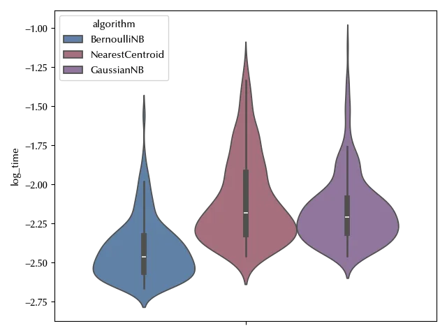
Since we already performed a similar analysis, we know that using the time as variable might cause some issue, and using its logarithm is better.

df['log_time'] = np.log(df['time'])

fig, ax = plt.subplots()
sns.violinplot(df, y='log_time', hue='algorithm', ax=ax)
fig.tight_layout()

We can now implement the model. In principle, we could (and, in my opinion, should) use a hierarchical model to perform the analysis. However, the small number of groups and subgroups would make this task hard, and we will simply use a linear model.

model = bmb.Model('log_time ~ algorithm + i + j',
                  data=df, categorical=['i', 'j', 'algorithm'])

idata = model.fit(**kwargs)

az.plot_trace(idata)
fig = plt.gcf()
fig.tight_layout()

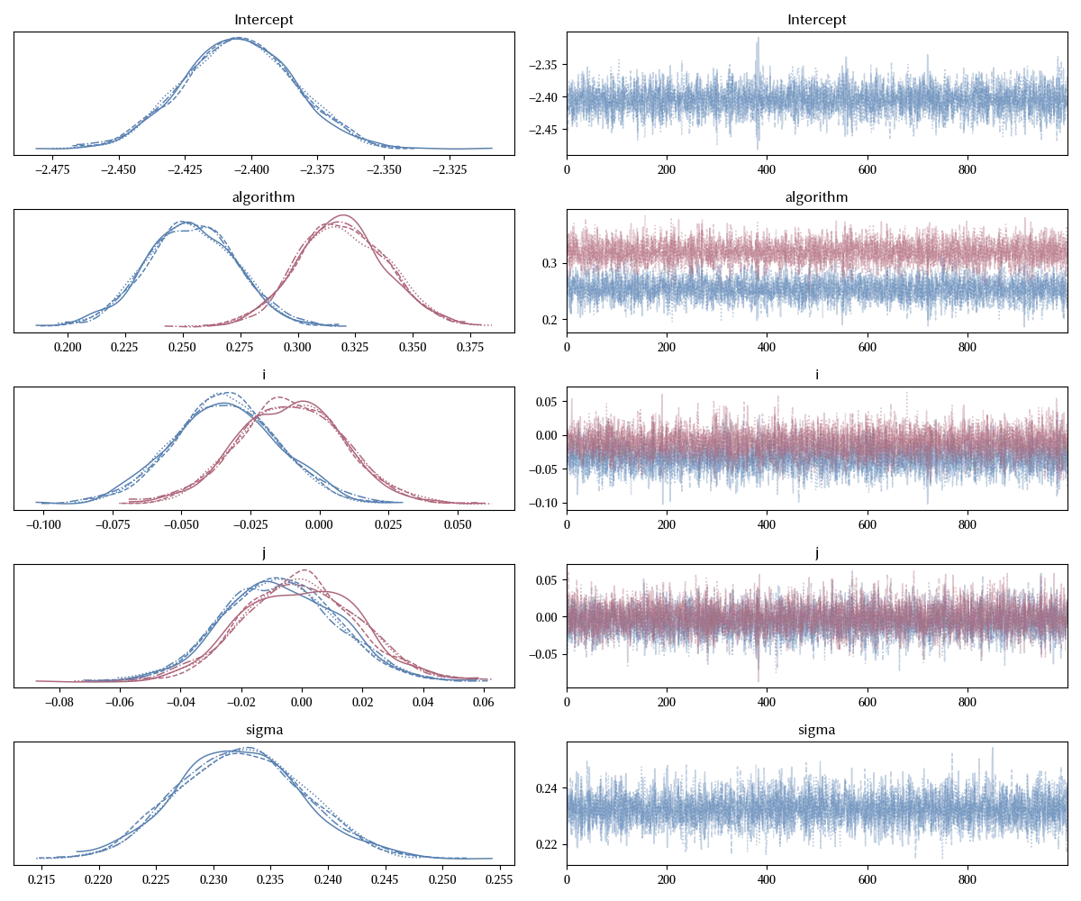
The trace looks decent, let us now take a look at our parameter of interest

az.plot_forest(idata, var_names=['algorithm'])
fig = plt.gcf()
fig.tight_layout()

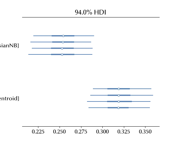
The Bernoulli Naive Bayes classifier is clearly faster with respect to the remaining algorithms.

Conclusions

We have seen how to run and analyze a latin square design. In the following posts, we will take a look at some more in-depth question related to experiment design.

The latin square design

Our experiment

Conclusions

Suggested readings