Full factorial design

In the previous post we discussed how to perform a completely randomized design experiment (CRD). In a CRD there is only one factor of interest, and we generally want to assess the effect of the different levels of that factor on the outcome.

There are however situations when the factors of interest are more than one. One common case is when you don’t know which factors are relevant for the outcome, and your aim is to clarify which are the factors that are relevant and which ones are irrelevant for the outcome. Another common thing you might want to do is to find the optimal setup for your experiment.

In a full factorial experiment, we have $k$ factors of interest, and we run the experiment by combining all the levels of all the factors. If we only perform one repetition, and assuming that we are considering an equal number of levels $n$ for each factor, then the number of runs is $n^k$. This number grows a lot as soon as $n$ grows, so a common strategy is to first fix $n=2$ for all the factor in order to discover which are the relevant factors. Only then we either fix the irrelevant factors or we randomize over them and increase the number of levels of the relevant factors (if more than two levels are possible) in order to optimize over them. A more modern approach, which will be discussed in a future post, is to dynamically look for the optimum value conditioning on the already observed values by using the so-called Gaussian Process optimization, but this is a rather advanced topic, and we will talk about this when discussing non-parametric models.

Let us first look at how to run a $2^k$ experiment, we will discuss how to generalize for larger $n$ in a later post.

A pipeline for ML optimization

Let us assume that we want to discover which is the optimal set of parameters to train a ML algorith with a given dataset. Let us assume that the algorithm allows for a large number of parameters. We will use a gradient boosting regressor for our problem, and we will take the Abalone dataset. As before, we will perform multiple train-test split, but this time we will not match over them. In order to show how to perform and analyze a full factorial example, we will instead randomize over the train-test split.

We will take consider the following combinations of factors:

loss: absolute error vs Huber
criterion: Friedman MSE vs squared error
learning rate: 0.25 and 0.75
max features: number of features or its square root.

Each combination will be tested with 50 different random train-test split.

import random
import time
import pandas as pd
import numpy as np
from ucimlrepo import fetch_ucirepo
from sklearn.ensemble import GradientBoostingRegressor
from sklearn.model_selection import train_test_split
from sklearn.metrics import r2_score, mean_absolute_error

dataset = fetch_ucirepo(id=1)

Xs = dataset.data.features
X = Xs
dummies = pd.get_dummies(Xs['Sex'])
X.drop(columns='Sex', inplace=True)

X = pd.concat([X, dummies], axis=1)
ys = dataset.data.targets.values.ravel()


loss_list = ['absolute_error', 'huber']
criterion_list = ['friedman_mse', 'squared_error']
learning_rate_list = [0.25, 0.75]
max_features_list = [None, 'sqrt']

combs = []

reps = 50
l = 0

for loss in loss_list:
    for criterion in criterion_list:
        for max_features in max_features_list:
            for learning_rate in learning_rate_list:
                for rep in range(reps):
                    state = np.random.randint(100000)
                    combs += [{'loss': loss,
                               'criterion': criterion,
                               'learning_rate': learning_rate,
                               'max_features': max_features,
                               'state': state, 'rep': rep, 'idx': l}]
                    l += 1


out = []
k = 0
random.shuffle(combs)
for comb in combs:

    Xtrain, Xtest, ytrain, ytest = train_test_split(X, ys, random_state=state)
    regr = GradientBoostingRegressor(loss=comb['loss'],
                                     criterion=comb['criterion'],
                                     learning_rate=comb['learning_rate'],
                                     max_features=comb['max_features'])
    regr.fit(Xtrain, ytrain)
    ypred = regr.predict(Xtest)
    score = mean_absolute_error(ytest, ypred)
    pars = comb
    pars.update({'score': score, 'ord': k})
    out.append(pars)
    k += 1
    print(k, len(combs), k/len(combs), score)

df = pd.DataFrame.from_records(out)

df.to_csv('full_factorial.csv')

Experiment analysis

Let us first of all import all the relevant libraries and the data.

import pandas as pd
import seaborn as sns
import numpy as np
import pymc as pm
import arviz as az
import bambi as bmb
from matplotlib import pyplot as plt

rng = np.random.default_rng(42)

kwargs = {'nuts_sampler': 'numpyro', 'random_seed': rng,
          'draws': 2000, 'tune': 2000, 'chains': 4, 'target_accept': 0.95}

df = pd.read_csv('full_factorial.csv')

df['max_features'] = df['max_features'].fillna('features')

df.head()

	Unnamed: 0	loss	criterion	learning_rate	max_features	state	rep	idx	score	ord
0	0	absolute_error	squared_error	0.75	features	99122	0	250	1.60952	0
1	1	huber	friedman_mse	0.75	sqrt	71432	42	592	1.68774	1
2	2	huber	squared_error	0.25	features	44912	31	631	1.56034	2
3	3	huber	squared_error	0.25	features	92911	20	620	1.55886	3
4	4	absolute_error	squared_error	0.25	features	49787	40	240	1.57739	4

Let us now prepare the data for the analysis. In order to have an idea of what are the relevant factors, we will first use a non-interacting model.

model_ni = bmb.Model('score ~ criterion + loss + max_features + learning_rate',
                     data=df, categorical=['criterion', 'loss', 'max_features'])

idata_ni = model_ni.fit(**kwargs)

az.plot_trace(idata_ni)
fig = plt.gcf()
fig.tight_layout()

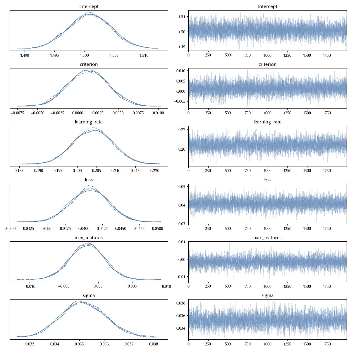
The trace of the non-interacting model

We immediately see that the only significant factors in this model are the loss and the learning rate. We have enough information in order to consider all the possible interaction terms, and this is what we will do. Building the fully interacting model is immediate with Bambi

model_int = bmb.Model('score ~ criterion * loss * max_features * learning_rate',
                      data=df, categorical=['criterion', 'loss', 'max_features'], )

idata_int = model_int.fit(**kwargs)

az.plot_trace(idata_int)
fig = plt.gcf()
fig.tight_layout()

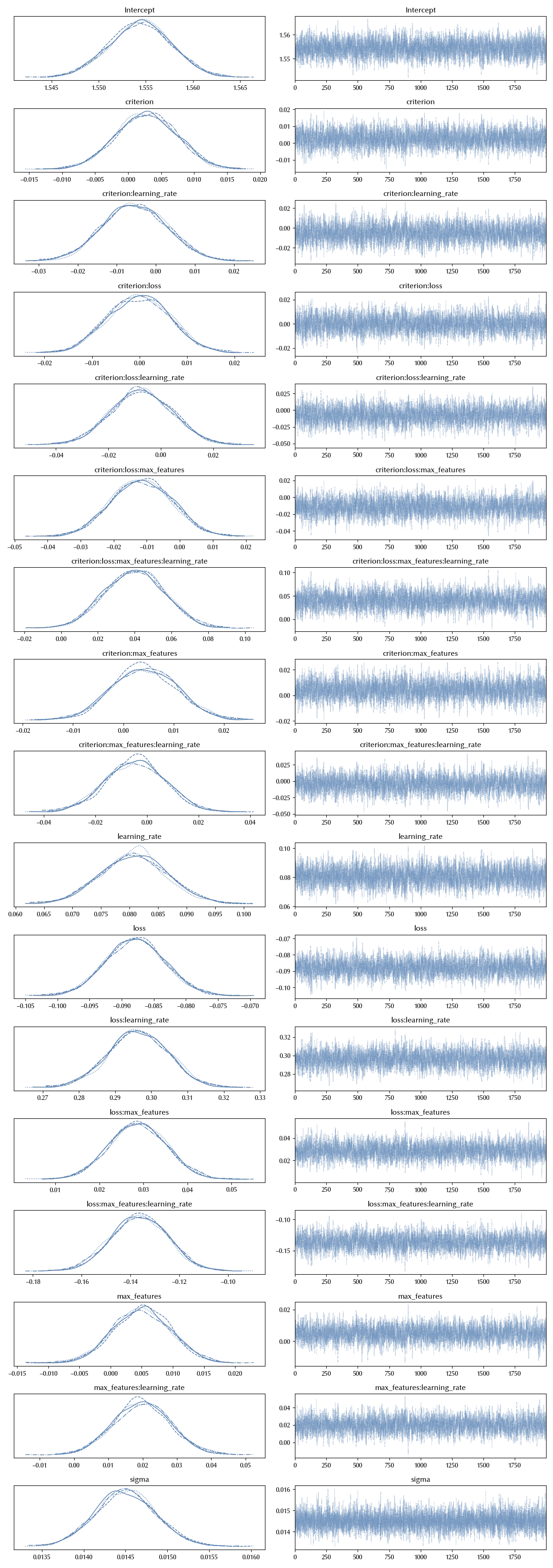
The trace of the fully interacting model

It is clear that, by only keeping the non-interacting terms, we were missing a lot of information.

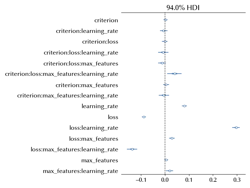
fig, ax = plt.subplots(figsize=(12, 9))
ax.axvline(x=0, color='k', ls=':')
az.plot_forest(idata, var_names=['beta'], ax=ax, combined=True)
fig.tight_layout()

Finding the optimal combination within the one in the above dataset can be done as follows

df_pred = df_ni.drop_duplicates()

model_int.predict(idata_int, data=df_pred, kind="response_params", inplace=True)

df_pred['mean_absolute_error'] = idata_int.posterior['mu'].mean(dim=('draw', 'chain')).values

df_pred['mean_absolute_error_std'] = idata_int.posterior['mu'].std(dim=('draw', 'chain')).values

df_pred.sort_values(by='mean_absolute_error', ascending=True)

	loss	criterion	max_features	learning_rate	mean_absolute_error	mean_absolute_error_std
2	huber	squared_error	features	0.25	1.56031	0.00203882
5	huber	friedman_mse	features	0.25	1.56084	0.00204077
15	huber	friedman_mse	sqrt	0.25	1.5655	0.00206221
10	huber	squared_error	sqrt	0.25	1.56654	0.00206114
7	absolute_error	friedman_mse	features	0.25	1.57463	0.00205604
4	absolute_error	squared_error	features	0.25	1.57605	0.00204244
60	absolute_error	friedman_mse	sqrt	0.25	1.5846	0.00202452
30	absolute_error	squared_error	sqrt	0.25	1.58915	0.00201078
0	absolute_error	squared_error	features	0.75	1.61377	0.00205295
11	absolute_error	friedman_mse	features	0.75	1.615	0.00205967
36	absolute_error	squared_error	sqrt	0.75	1.63457	0.00204341
18	absolute_error	friedman_mse	sqrt	0.75	1.63491	0.00204379
1	huber	friedman_mse	sqrt	0.75	1.69584	0.00206499
14	huber	squared_error	sqrt	0.75	1.70833	0.00205859
6	huber	squared_error	features	0.75	1.74248	0.00204959
17	huber	friedman_mse	features	0.75	1.74938	0.00203594

The choice of the criterion has no impact on the error, and we can be quite sure that the optimal setup has the Huber loss, probably with the “features” number of max_features, and a small learning rate.

We stress that the learning rate is a continuous variables, so we cannot only use two values to find the minimum score. We will discuss this kind of problem in a future post.

We can finally take a look at the average predictions

fig, ax = plt.subplots(ncols=2, nrows=2)
bmb.interpret.plot_predictions(idata=idata_int, model=model_int, conditional='learning_rate', ax=ax[0][0])
ax[0][0].set_xlim([0.25, 0.75])

bmb.interpret.plot_predictions(idata=idata_int, model=model_int, conditional='criterion', ax=ax[0][1])
bmb.interpret.plot_predictions(idata=idata_int, model=model_int, conditional='loss', ax=ax[1][0])
bmb.interpret.plot_predictions(idata=idata_int, model=model_int, conditional='max_features', ax=ax[1][1])
fig.tight_layout()

The plot of the average predictions

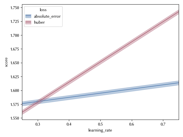
Notice that, from the above plot, it looks like the score of the predictions for the Huber loss are higher than the ones obtained by using the absolute error. This only happens once we integrate over the remaining factors, while we are interested in conditioning over them, since we are looking for the optimal value. We can convince ourselves of the above statement by looking at the following figure:

fig, ax = plt.subplots()
bmb.interpret.plot_predictions(idata=idata_int, model=model_int,
                               conditional={'learning_rate': [0.25, 0.75],
                                            'loss': ['absolute_error', 'huber']},
                              ax=ax)
ax.set_xlim([0.25, 0.75])
fig.tight_layout()

The conditional predictions

Conclusions

We have seen how to run and analyze a full factorial experiment with binary outcomes. This method can be seen as a form of cross-validated grid search, but in this case the execution order is random rather than deterministic. Moreover, by using the above method, we are also able to take the performance variance into account, while the more traditional grid search only considers the average performances.

A pipeline for ML optimization

Experiment analysis

Conclusions

Suggested readings